
Machine Learning for Time Series Forecasting:
While traditional statistical methods (like ARIMA, SARIMA) have been widely used machine learning (ML) offers increased flexibility, especially when working with non-linear patterns, external variables, and large datasets common in the fashion retail industry.
Why Use Machine Learning for Time Series Forecasting?
- Handles complex patterns and multiple variables
- Can scale with big data (e.g., thousands of products/SKUs)
- Can model non-linear trends and interactions
- Useful for real-time forecasting
Python Implementation for Time Series using Machine Learning Model:
# Import Necessary Libraries
import pandas as pd
import numpy as np
import matplotlib.pyplot as plt
import seaborn as sns
from sklearn.ensemble import RandomForestRegressor, GradientBoostingRegressor
import xgboost as xgb
import lightgbm as lgb
from sklearn.metrics import mean_squared_error
from sklearn.model_selection import train_test_split
from warnings import filterwarnings
filterwarnings('ignore')
# Loading Data
df = pd.read_csv('/content/Time_series.csv')
df['date'] = pd.to_datetime(df['date'])
df.set_index('date', inplace=True)
# Feature engineering
df['lag_1'] = df['sales'].shift(1)
df['lag_7'] = df['sales'].shift(7)
df['rolling_mean_7'] = df['sales'].rolling(window=7).mean()
df['day_of_week'] = df.index.dayofweek
df.dropna(inplace=True)
# Define features and target
X = df[['lag_1', 'lag_7', 'rolling_mean_7', 'day_of_week']]
y = df['sales']
# Train-test split
X_train, X_test, y_train, y_test = train_test_split(X, y, shuffle=False, test_size=0.2)
# Models dictionary
models = {
'Random Forest': RandomForestRegressor(n_estimators=100, random_state=42),
'Gradient Boosting (sklearn)': GradientBoostingRegressor(n_estimators=100, random_state=42),
'XGBoost': xgb.XGBRegressor(n_estimators=100, random_state=42, objective='reg:squarederror'),
'LightGBM': lgb.LGBMRegressor(n_estimators=100, random_state=42)
}
# Fit models and collect predictions
predictions = {}
for name, model in models.items():
model.fit(X_train, y_train)
preds = model.predict(X_test)
predictions[name] = preds
# Evaluation and visualization
results = pd.DataFrame(predictions, index=y_test.index)
results['Actual'] = y_test
# Calculate RMSE for each model
rmse_scores = {name: np.sqrt(mean_squared_error(y_test, preds)) for name, preds in predictions.items()}
# Plot with RMSE in legend
plt.figure(figsize=(14, 8))
for name in models:
plt.plot(results.index, results[name], label=f"{name} (RMSE: {rmse_scores[name]:.2f})")
plt.plot(results.index, results['Actual'], label='Actual', linewidth=3, linestyle='--', color='black')
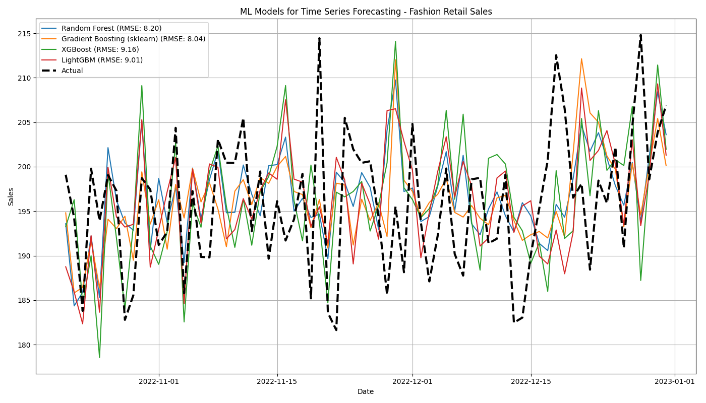
plt.title('ML Models for Time Series Forecasting - Fashion Retail Sales')
plt.xlabel('Date')
plt.ylabel('Sales')
plt.legend()
plt.grid(True)
plt.tight_layout()
plt.savefig('ML_models.png')
plt.show()
Let's move to Time Series Forecasting - Deep Learning Model>>>
