Nowadays, data is everywhere in this digital age! Have you ever think how all this data is stored and managed? The answer is Databases! And to interact with databases, we use query language like SQL (Structured Query Language).
Database:
A database is an organized collection of data that allows easy access, management, and retrieval. Imagine a library where books are stored systematically so you can easily find what you need. Similarly, databases store data in a structured way.
Types of Databases:
- Relational Databases – Data is stored in tables with rows (tuples) and columns (attributes) (SQL-based)
- Non-relational databases (NoSQL) Databases – Flexible structure (key-value, documents, graphs)
DBMS(Data Base Management System):
The software that is used to manage databases is called Database Management System. DBMS allows users to create, read, update, and delete data in the database.
This blog will focus on Relational Databases, where SQL is used.
RDBMS(Relational Database Management System):
RDBMS is a software which is used to manage Relational databases in which data is stored in the form of rows and columns which can be easily retrieved, managed and updated.
Type of Relational Database Management Systems (RDBMS) :
1. Enterprise & Open-Source RDBMS
| RDBMS | Description |
|---|---|
| MySQL | Open-source, widely used in web applications (e.g., WordPress, Facebook). |
| PostgreSQL | Open-source, highly extensible, supports advanced SQL features and NoSQL-like operations. |
| Microsoft SQL Server (MSSQL) | Developed by Microsoft, it is used in enterprise applications with deep integration into Windows and Azure. |
| Oracle Database | A powerful, enterprise-grade RDBMS used in large-scale applications. |
| IBM Db2 | An enterprise-level RDBMS used for high-performance applications. |
| MariaDB | A MySQL-compatible RDBMS is often considered a drop-in replacement with additional features. |
| Firebird | Open-source RDBMS with advanced SQL support. |
2. Cloud-Based RDBMS
| RDBMS | Description |
|---|---|
| Google Cloud Spanner | A globally distributed RDBMS with strong consistency. |
| Amazon RDS (Relational Database Service) | Supports MySQL, PostgreSQL, SQL Server, Oracle, and MariaDB on AWS. |
| Azure SQL Database | A managed cloud version of Microsoft SQL Server. |
3. Embedded RDBMS
| RDBMS | Description |
|---|---|
| SQLite | A lightweight, serverless database used in mobile and embedded systems. |
| H2 Database | A Java-based, lightweight RDBMS often used in testing and development. |
4. Specialized RDBMS
| RDBMS | Description |
|---|---|
| CockroachDB | A distributed SQL database with strong consistency and fault tolerance. |
| Percona Server | A high-performance alternative to MySQL and MariaDB. |
SQL (Structured Query Language):
It is the standard language used to interact with relational databases. It helps you store, retrieve, update, and delete data efficiently. SQL works with popular databases like MySQL, PostgreSQL, SQLite, SQL Server, and Oracle.
All tables in SQL need to have their ‘schema’ defined at the moment of creation.
”In SQL, a schema is a logical container that holds database objects such as tables, views, indexes, stored procedures, and functions.”
Functions of SQL:
• Create new databases and tables.
• Executes queries against a database.
• Retrieve, update, and insert records into a database.
• Create stored procedures and views in a database.
• Set permissions on tables, procedures, and views.
SQL Commands:
To interact with databases and SQL commands are divided into several categories based on their function. Here are the main types of SQL commands:
1. Data Definition Language (DDL)
- DDL commands are used to define and manage the structure of a database.
- They allow you to create, modify, and delete database objects like tables, indexes, and views.
- Common DDL commands include:
CREATE: Creates a new database object (e.g., table, index).ALTER: Modifies an existing database object.DROP: Deletes a database object.TRUNCATE: Removes all data from a table but keeps the table structure.COMMENT: Adds comments to database objects.RENAME: Renames a database object.
2. Data Manipulation Language (DML)
- DML commands are used to work with the data within a database.
- They allow you to insert, update, delete, and retrieve data from tables.
- Common DML commands include:
INSERT: Adds new rows to a table.UPDATE: Modifies existing data in a table.DELETE: Removes rows from a table.SELECT: Retrieves data from one or more tables.
3. Data Query Language (DQL)
- DQL commands are specifically used for querying data from a database.
- The primary DQL command is
SELECT, which allows you to specify the data you want to retrieve and how it should be organized. - While some sources consider DQL as a separate category, it is often considered a subset of DML since
SELECTis used to manipulate data retrieval.
4. Data Control Language (DCL)
- DCL commands are used to manage user access and permissions within a database.
- They allow you to grant and revoke privileges to users, controlling what actions they can perform.
- Common DCL commands include:
GRANT: Gives specific permissions to users.REVOKE: Removes permissions from users.
5. Transaction Control Language (TCL)
- TCL commands are used to manage transactions within a database.
- Transactions are sequences of SQL operations that are treated as a single unit of work.
- TCL commands allow you to control the start, commit, and rollback of transactions.
- Common TCL commands include:
COMMIT: Saves all changes made during the current transaction.ROLLBACK: Reverts all changes made during the current transaction.SAVEPOINT: Sets a point within a transaction to which you can roll back.
Database Environment:
We need a database environment to write SQL queries
1. Database Management Systems (DBMS):
Most databases provide built-in tools for writing and running SQL queries:
- SQL Server (Microsoft SQL Server)
- Use SQL Server Management Studio (SSMS)
- Write queries in the Query Editor and execute them
- MySQL
- Use MySQL Workbench (Graphical User Interface)
- Use the MySQL Command Line Client
- PostgreSQL
- Use pgAdmin (GUI)
- Use the psql command-line tool
- Oracle
- Use SQL*Plus (Command Line)
- Use Oracle SQL Developer (GUI)
2. Online SQL Editors
If you don’t want to install a database, you can use online platforms like:
- SQL Fiddle
- DB Fiddle
- Mode Analytics
- W3Schools SQL Tryit
3. Programming Languages (Using SQL in Code)
You can write SQL queries inside programming languages using database connectors:
- Python (with sqlite3, PyMySQL)
- R (with DBI and RSQLite)
- Java (with JDBC)
- js (with mysql or pg libraries)
4. Command Line Interface (CLI)
If you prefer working in a terminal:
- MySQL: mysql -u root -p
- PostgreSQL: psql -U username -d database
- SQL Server: sqlcmd -S server_name -U username -P passwordDB Browser for SQLite
5. DB Browser(SQLite)
If you are a beginner you can use DB Browser for SQLite which is a free and open-source GUI tool that allows you to create, edit, and manage SQLite databases without writing complex SQL commands. It is useful for developers, data analysts, and anyone who needs to interact with SQLite databases visually.
I will describe 3 environments how to set up:
01. MySQL Workbench:
- Download: Go to the official MySQL website (https://dev.mysql.com/downloads/workbench/), choose your OS, and download the installer.
- Install: Run the installer and follow the instructions.
- Connect: Open MySQL Workbench, create a new connection, enter your MySQL server details (hostname, port, username, password), and test the connection.
- Use: Open a query tab to write and execute SQL queries, use the visual designer, data editor, or other tools. You’ll need a MySQL server running separately.
02. DB Browser for SQLite:
- Download: Go to the official website https://sqlitebrowser.org/dl/ choose your OS, and download the installer.
- Install: Run the installer and follow the instructions.
- Open: Search in the Windows menu for DB Browser for SQLite and open it. Click the ‘Open Database’ button to load the database
- Browse Data: Explore different tables under the ‘Browse Data’ tab.
- Write Query: Move to the ‘Execute SQL’ tab to write a query
03. PyMySQL to Connect Python to MySQL:
#Install
! pip install pymysql

#Import
import pymysql

# Connect to MySQL
connection = pymysql.connect(
    host='localhost',
    user='root',
    password='your_password',
    database='your_database'
)

# Execute a query
query = "select * from dataset_list "

pd.read_sql(query,connection)
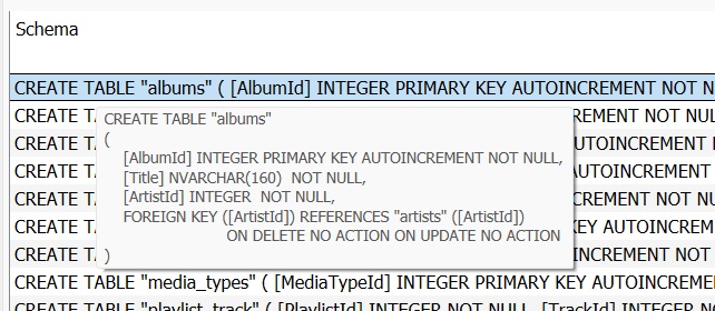
Schema:
A schema is a logical container that organizes database objects such as tables, views, indexes, procedures, and functions. It provides a way to group related objects together and manage permissions at a higher level. All tables in SQL need to have their ‘schema’ defined at the moment of creation. This means, that for each attribute (column), one needs to know the type of data that will be entered.
Constraints:
Constraints are rules applied to each attribute in a database table to restrict data integrity and ensure the accuracy and reliability of the data. Constraints can be applied during the creation of a table or can be added later
Common Types of Constraints in SQL:
- NOT NULL: Ensures that a column cannot have a NULL value.
- UNIQUE: Ensures that all values in a column are distinct.
- PRIMARY KEY: The unique identifier for each row in a table. There can only be one PRIMARY KEY in a table, and it also needs to be NOT NULL and UNIQUE.
- COMPOUND (COMPOSITE) KEY: Consists of two or more columns that together uniquely identify a row.
- FOREIGN KEY: Column (or set of columns) that references a Primary Key in another table, this ensures that every Primary Key in our table must exist in the referencing table
- CHECK: Ensures that the values in a column satisfy a specific condition.
- DEFAULT: Sets a default value for a column when no value is specified.
- AUTO INCREMENT: automatically add 1 to a value when new records
are added to a table.
Example:
-- Using Primary key

CREATE TABLE Employees (
    EmployeeID INT PRIMARY KEY,  -- Primary key constraint
    FirstName VARCHAR(50) NOT NULL,  -- NOT NULL constraint
    LastName VARCHAR(50) NOT NULL,
    Email VARCHAR(100) UNIQUE,  -- UNIQUE constraint
    Salary DECIMAL(10, 2) CHECK (Salary > 0),  -- CHECK constraint
    DepartmentID INT,
    FOREIGN KEY (DepartmentID) REFERENCES Departments(DepartmentID)  -- FOREIGN KEY constraint
);


-- Using compound key

CREATE TABLE Employees (
    EmployeeID INT,
    DepartmentID INT,
    FirstName VARCHAR(50) NOT NULL,  -- NOT NULL constraint
    LastName VARCHAR(50) NOT NULL,
    Email VARCHAR(100) UNIQUE,  -- UNIQUE constraint
    Salary DECIMAL(10, 2) CHECK (Salary > 0),  -- CHECK constraint
    PRIMARY KEY (EmployeeID, DepartmentID),  -- Compound primary key
    FOREIGN KEY (DepartmentID) REFERENCES Departments(DepartmentID)  -- FOREIGN KEY constraint
);
Creating, modification & joining Database in MySQL (with Example):
-- Create employee database
create database employee;

-- Create datamites database
create database datamites;

-- How to see all the available databases
show databases;

-- Delete datamites database
drop database datamites;

-- switch to employee database
use employee;

-- Create employee_data table with emp_id,emp_name , emp_age,emp_salary ,join_date,emp_job

create table employee_data
(emp_id int ,
emp_name varchar(20),
emp_age int ,
emp_salary int,
join_date date,
emp_job varchar(25));

-- See all the avialable tables in employee database
show tables;

-- how to see the structure of table
desc employee_data;

-- How to view table
select * from employee_data;

-- How to delete a table;
drop table employee_data;

-- create employee_details table
create table employee_details
(emp_id varchar(10) primary key,
emp_name varchar(20) not null ,
emp_job varchar(25) not null,
emp_salary int default 20000,
join_date date ,
emp_age int check(emp_age>20));

desc employee_details;
select * from employee_details;

-- insert single record into a table
insert into employee_details values
("ES0001","Rana","HR",40000,"2023-02-24",30);

-- insert multiple record into table
insert into employee_details values
("ES0002","Sujon","Manager",50000,"2022-04-23",40),
("ES0003","Masud","Analyst",70000,"2022-06-20",27),
("ES0004","Raisa","Engineer",65000,"2021-12-11",30),
("ES0005","Armaan","Tech manager",80000,"2023-01-13",40);

-- insert record with 5 values ---> we end up with error
insert into employee_details values
("ES0007","Musfiq","Teacher","2023-02-24",30);

-- insert values into specific columns --> columns which are not specified will take null values.
insert into employee_details(emp_id,emp_name,emp_job,emp_salary) values
("ES0009","Jeevitha","DataScientist",80000);

-- In this query emp_salary will take default value as 20000 , emp_job,join_date will take null values.
insert into employee_details(emp_id,emp_name,emp_job) values
("ES0008","Samita","Professor");

-- This query will throw an error because emp_id ,emp_name and emp_job cannot be empty
insert into employee_details(emp_salary,emp_age,join_date) values
(10000,30,"2022-02-23");

-- This query will throw an error because emp_age should be greater than 20 but we have taken 18.
insert into employee_details values
("ES0010","Anjan","HR",50000,"2023-02-24",18);

select * from employee_details;

-- Modification

-- change employee salary and employee age to 80000 and 35 of first record.
update employee_details set emp_salary=80000 ,emp_age=35 where emp_id="ES0001";

-- change job of Raisa to SalesManager
update employee_details set emp_job="SalesManager" where emp_id="ES0004";

-- update age of Samita and Rana to 30
update employee_details set emp_age=30 where emp_name="Jeevitha" or emp_name="Smitha";

select * from employee_details;

-- delete information related to Rana
delete from employee_details where emp_name="Rana";

-- delete record related to Samita
delete from employee_details where emp_name="Samita";

set autocommit=off;
-- delete records related to Armaan and Musfiq
delete from employee_details where emp_name="Armaan" or emp_name="Musfiq";

Rollback;

update employee_details set emp_age=100 where emp_id="ES0001";
Rollback;
select * from employee_details;
-- Alter statement and add is used to create new columns.
-- add new field emp_experience
alter table employee_details add emp_experience int unique;

-- create new fields like class1 and class2
alter table employee_details add class1 varchar(10) , add class2 date;

update employee_details set class1="python",class2="2023-02-23";
update employee_details set emp_experience=4 where emp_id="ES0001";

-- Delete emp_experience
alter table employee_details drop column emp_experience;

-- Delete class1 and class2 fields
alter table employee_details drop class1,drop class2;

select * from employee_details;

-- How to see structure of table
desc employee_details;

-- change data type of emp_name to varchar(100)
alter table employee_details modify emp_name varchar(100);

-- change data type of salary to numeric
alter table employee_details modify emp_salary numeric;

-- change emp_name  to name_of_employee
alter table employee_details rename column emp_name to name_of_employee;

desc employee_details;

-- change employee_details name employee_data1
alter table employee_details rename to employee_data1;
SQL COMMANDS:
- SQL is case-insensitive
- The standard way is to use SQL commands in all caps
- Queries are ended with a semi-colon, ‘;’
- SQL comments are created with ‘–’.
- If we use ‘*’ wildcard in place of an attribute that translates to “all columns”
- Optional AS to rename a table temporarily
- WHERE a Boolean condition is TRUE (or FALSE if using the NOT optional).
- We can use WHERE expressions with AND or OR.
- A comma, ‘,’ is used when selecting multiple attributes (e.g. SELECT
<column1>, <column2>, <column3>).
SELECT <attribute> FROM <TableName> [AS <Name>] WHERE [NOT] <condition>;
Some common commands:
- Fetching all the records from the table
- SELECT < * > FROM < table name > ;
- Fetching a subset of columns
- SELECT < column > FROM < table name > ;
- SELECT < column1 >,< column2 > FROM < table name > ;
- Fetching unique records or values from the table.
- SELECT DISTINCT <column> FROM < table name > ;
- Aggregate functions are used to perform the calculations on multiple rows of a single column and return a single value. Types of Aggregate functions as below:
- Returns only one row with the total number of records.
- SELECT <COUNT(column)> FROM < table name > ;
- Returns only one row with the mean average for the given numeric column.
- SELECT <AVG(column)> FROM < table name > ;
- Returns only one row with the sum for the given numeric column.
- SELECT <SUM(column)> FROM < table name > ;
- Returns only one row with the minimum value from the given numeric column.
- SELECT <MIN(column)> FROM < table name > ;
- Returns only one row with the maximum value from the given numeric column.
- SELECT <MAX(column)> FROM < table name > ;
- Returns only one row with the total number of records.
- SQL Aliases are used to give temporary names for columns and tables.
- SELECT <column_name> AS <alias_name> FROM < table name >;
- WHERE clause is used to filter records based on condition.
- SELECT * FROM < table name > WHERE <condition> ;
- Conditions are of two types:
- Comparison : = , > ,< >= ,<= ,!=
- Logical: AND, OR, NOT
- SELECT * FROM < table name > WHERE <condition 1> AND <condition 2>;
- SELECT * FROM < table name > WHERE <condition 1> OR <condition 2>;
- SELECT * FROM < table name > WHERE NOT <condition >;
- ORDER BY keyword is used to sort the records in Ascending or descending order.
- SELECT * FROM < table name > WHERE <condition > ORDER BY <column> ASC/DESC;
- IS NULL/IS NOT NULL are used to check whether null values exist in the table.
- SELECT * FROM < table name > WHERE <column1 > IS NULL;
- SELECT * FROM < table name > WHERE <column1 > IS NOT NULL;
- LIMIT is used to return the specified number of records.
- SELECT * FROM < table name > WHERE <condition> LIMIT <value>;
- IN is used to return records where some specific values are present.
- SELECT * FROM < table name > WHERE <column1> IN (val1 ,val2,val3);
- BETWEEN is used to return records within a certain range. It can be values, dates, or text.
- SELECT * FROM < table name > WHERE <column1> BETWEEN <val1> AND <val2>;
- LIKE is used to return records based on the pattern.
- SELECT * FROM < table name > WHERE <column1> LIKE <PATTERN>;
- ‘%’ – It represents zero, one or multiple characters.
- ‘ _ ‘ – It is used to represent one or a single character.
- ‘a%’ – It returns values that start with a (we can use our required letter).
- ‘%a’ – It returns values that end with a (we can use our required letter).
- ‘%a%’ – It returns values that have a in any position (we can use our required letter).
- ‘b%a’ – It returns values that start with b and end with a (we can use our required letter).
- ‘_a%’ – It returns values that have a in the second position.
- ‘%a_’ – It returns values that have a in the second last position.
- ‘__a%’ – It returns values that have a in the third position.
- ‘%a__’ – It returns values that have a in the third last position.
- same for the fourth, fifth & so on
- GROUP BY is used to arrange identical data into groups with the help of aggregate functions.
- SELECT column1 , function(column2) FROM <table_name> GROUP BY <column1>;
- HAVING clause is used to filter the result obtained by the group by clause based on specific conditions. HAVING clause is used with aggregate functions (like COUNT(), SUM(), AVG(), etc.), not for filtering individual rows . We need to use GROUP BY first and HAVING to filter grouped results.
- SELECT column1 ,function(column2) FROM <table_name> GROUP BY <column1 > HAVING <condition> ORDER BY <column2>;
- Rules to use HAVING:
- The group by clause is used with select statement.
- Group by is placed before having clause.
- Group by clause is placed before order by.
- Having clause is placed before order by.
- Conditions are specified in having clause
- SUBQUERY is a query within another SQL query. The outer query is the main query and the inner query is the subquery.
- Subquery must be enclosed within parentheses.
- Order by cannot be used in a subquery.
- Between operators cannot be used.
- A subquery can have only single column in subquery.
- SELECT columns FROM table
WHERE column_name <expression operator>
(SELECT column_name FROM table_name WHERE <condition>);
| Operator | Description |
| = | Equal to |
| != or <> | Not equal to |
| > | Greater than |
| < | Less than |
| >= | Greater than or equal to |
| <= | Less than or equal to |
| IN | Matches any value in the subquery result |
| NOT IN | Excludes values from the subquery result |
| EXISTS | Returns true if the subquery has at least one row |
| NOT EXISTS | Returns true if the subquery returns no rows |
- JOINS are used to combine two tables based on
common column, and selects records that have matching
values in these columns.- INNER JOIN or JOIN: Inner join or join returns those records which have
matching values in both tables.- SELECT <column_names> FROM Table1
INNER JOIN Table2
ON Table1.matching_column=Table2.matching_column ; - SELECT <column_names> FROM Table1
INNER JOIN Table2
USING(matching_column) ; - SELECT <column_names> FROM Table1
JOIN Table2
ON Table1.matching_column=Table2.matching_column ; - SELECT <column_names> FROM Table1
JOIN Table2
USING(matching_column) ;
- SELECT <column_names> FROM Table1
- LEFT JOIN: Left join returns all the records from left table and
also matching records from right table.- SELECT <column_names> FROM Table1
LEFT JOIN Table2
ON Table1.matching_column=Table2.matching_column ; - SELECT <column_names> FROM Table1
LEFT JOIN Table2
USING(matching_column) ;
- SELECT <column_names> FROM Table1
- RIGHT JOIN: Right join returns all the records from right table and also
matching records from left table- SELECT <column_names> FROM Table1
RIGHT JOIN Table2
ON Table1.matching_column=Table2.matching_column ; - SELECT <column_names> FROM Table1
RIGHT JOIN Table2
USING(matching_column) ;
- SELECT <column_names> FROM Table1
- FULL OUTER JOIN: Full outer join returns all the records from both the
tables.- SELECT<column_names> FROMTable1
LEFT JOIN Table2
ON Table1.matching_column=Table2.matching_column
UNION
SELECT<column_names> FROMTable1
RIGHT JOIN Table2
ON Table1.matching_column=Table2.matching_column; - SELECT<column_names> FROMTable1
LEFT JOIN Table2
USING(matching_column)
UNION
SELECT<column_names> FROMTable1
RIGHT JOIN Table2
USING(matching_column) ; - SELECT<column_names> FROMTable1
FULL OUTER JOIN Table2
ON Table1.matching_column=Table2.matching_column;
- SELECT<column_names> FROMTable1
- CROSS JOIN: The cross join returns all the records from both the tables.
- SELECT column_name(s) FROM <Table 1> CROSS JOIN <Table 2>
- INNER JOIN or JOIN: Inner join or join returns those records which have
- WINDOW FUNCTIONS: A window function performs calculations for each row using other rows in a dataset. Unlike GROUP BY, window functions do not collapse rows but instead create a “window” of related records for calculations.
- Window functions require OVER() to define the “window” (the set of rows over which the function operates).
- OVER CLAUSE: Over clause defines the partitioning and ordering of rows for the given functions. Over clause accepts three arguments:
- Partition by: Divides the query result into sets. The window function is applied over each partition.
- Order by: Define the logical order of the rows
- Rows or range: Further limits the rows within the partition by specifying start and end points within the partitions
- Types of Window functions:
- Aggregate functions: avg, sum, count, min, max
- Ranking functions: row_number, rank, dense_rank
- Analytic functions: first_value , last value
- SELECT * ,aggregate_function(column) OVER(PARTITION BY column ORDER BY column) AS alias FROM table_name;
Examples for the above SQL commands :
-- Fetching all the records from the table 'employees'
SELECT *  FROM employees;

-- Fetching all the records from one column 'Country' of the table 'employees'
SELECT Country FROM employees;

-- Fetching all the records from two columns 'Country','City' of the table 'employees'
SELECT Country,City FROM employees;
-- Similarly we can fetch record from any numbers of columns

-- Fetching unique records of 'City' from the table 'employees'
SELECT DISTINCT(City) FROM employees;

-- Finding total number of records from 'City' of the table 'employees'
SELECT COUNT(City) FROM employees;

-- Finding average of column 'Total' from table  'invoices'
SELECT AVG(Total) FROM invoices;

-- Finding minimum value of column 'Total' from table  'invoices'
SELECT MIN(Total) FROM invoices;

-- Finding maximum value of column 'Total' from table  'invoices'
SELECT MAX(Total) FROM invoices;

-- Creating temporary column & giving a name
SELECT DISTINCT(Country) AS Country_list FROM customers;

-- Creating new table & giving a name
CREATE TABLE StateCountryCity AS SELECT State,Country,City  FROM customers;

-- Using WHERE clause
SELECT * FROM invoices WHERE BillingCity = 'London';

SELECT * FROM invoices WHERE BillingCity = 'London' AND BillingPostalCode = 'N1 5LH';

SELECT * FROM invoices WHERE BillingCity = 'London' OR BillingPostalCode = 'N1 5LH';

SELECT * FROM invoices WHERE NOT BillingCity = 'London';

SELECT * FROM invoices WHERE BillingCity != 'London';

SELECT * FROM invoices WHERE Total < 1;

SELECT * FROM invoices WHERE Total > 10;

SELECT * FROM invoices WHERE Total <= 1.98;

SELECT * FROM invoices WHERE Total >= 13.86;

SELECT * FROM invoices WHERE Total = 13.86;

SELECT * FROM invoices WHERE Total != 13.86;

-- Using  ORDER BY
SELECT * FROM invoices ORDER BY Total ASC;

SELECT * FROM invoices ORDER BY Total DESC;

-- Using IS NULL
SELECT * FROM invoices WHERE BillingPostalCode IS NULL;

-- Using IS NOT NULL
SELECT * FROM invoices WHERE BillingPostalCode IS NOT NULL;

-- Using LIMIT to get top 10 rows
SELECT * FROM invoices ORDER BY Total DESC LIMIT 10;

-- Using IN to get records where specified values present
SELECT * FROM invoices WHERE BillingCountry IN ('Austria','USA','Chile');

-- Using BETWEEN to get record from specified  range
SELECT * FROM invoices WHERE Total BETWEEN 8 AND 15;

-- Using LIKE to get match values
SELECT * FROM invoices WHERE BillingCountry LIKE 'U%';

SELECT * FROM invoices WHERE BillingCountry LIKE '%s';

SELECT * FROM invoices WHERE BillingCountry LIKE '%r%';

SELECT * FROM invoices WHERE BillingCountry LIKE 'B%l';

SELECT * FROM invoices WHERE BillingCountry LIKE '_r%';

SELECT * FROM invoices WHERE BillingCountry LIKE '%n_';

-- Using GROUP BY
SELECT BillingCountry,SUM(Total) FROM invoices GROUP BY BillingCountry;

-- Using HAVING
SELECT BillingCountry,SUM(Total)
FROM invoices
GROUP BY BillingCountry
HAVING SUM(Total)>100 ORDER BY SUM(Total) DESC; --ORDER BY can be skipped

-- Using subquery
SELECT * FROM invoices
WHERE BillingCountry IN
(SELECT BillingCountry FROM invoices WHERE CustomerId <5);

-- Using INNER JOIN
SELECT * FROM invoices
INNER JOIN customers
ON invoices.CustomerId = customers.CustomerId;

-- Using LEFT JOIN
SELECT * FROM invoices
LEFT JOIN customers
ON invoices.CustomerId = customers.CustomerId;

-- Using RIGHT JOIN
SELECT * FROM invoices
RIGHT JOIN customers
ON invoices.CustomerId = customers.CustomerId;

-- Using FULL OUTER JOIN
SELECT * FROM invoices
FULL OUTER JOIN customers
ON invoices.CustomerId = customers.CustomerId;

-- Using OVER()
SELECT *, SUM(Total)
OVER(PARTITION BY BillingCountry )
AS Countrysum FROM invoices;
