Semi Supervised Machine Learning

Semi-Supervised Machine Learning

• Semi-Supervised Machine Learning is a class of machine learning techniques that falls between supervised and unsupervised learning.
• It uses a small amount of labeled data and a large amount of unlabeled data to train models.
• Unlabeled data can provide structure and context, while labeled data provides specific guidance.

Importance of Semi-Supervised Learning

• In the real world, data is abundant, but labels are expensive. Whether it’s tagging thousands of images, labeling medical records, or categorizing customer feedback, creating labeled datasets often requires significant time, cost, and expertise.

• Semi-Supervised Machine Learning (SSML) offers a solution: it uses a small amount of labeled data and a large amount of unlabeled data to build models that are more accurate than purely unsupervised learning and more economical than fully supervised learning.

How Semi-Supervised Learning Works

The core idea of Semi-Supervised Learning is as follows:

1. Start with a small labeled dataset to establish an initial model.
2. Use this model to predict labels (Pseudo labels) for the unlabeled data.
3. Incorporate these Pseudo labels, often with confidence thresholds into the training set.
4. Iteratively refine the model, improving accuracy over time.

This process combines the structure discovery of unsupervised learning with the guidance of supervised learning.

Fundamental Assumptions in Semi-Supervised Learning

Semi-supervised learning assumes that unlabeled data must be relevant and informative for the task. It relies on the idea that the input distribution p(x) holds clues about the label distribution p(y∣x), a conditional probability of a given data point (x) which belongs to a certain class (y). Using irrelevant unlabeled data can decrease model performance, so it is essential to make correct assumptions. Some fundamental assumptions are as below:

1. Cluster Assumption

• Data tends to form discrete clusters, and points in the same cluster share the same label.
• This is why graph-based and clustering-based SSML methods work well — they spread labels across clusters.

2. Smoothness Assumption

• Points that are close together in the feature space are likely to have the same label.
• For example, if two product descriptions have very similar wording, they probably belong to the same category.

3. Distributional Similarity Assumption

• The distribution of labeled data is representative of the unlabeled data.
• If labeled data comes from a different distribution (e.g., labeling only simple cases but leaving hard cases unlabeled), SSML performance can degrade.

4. Manifold Assumption

• High-dimensional data actually lies on a lower-dimensional manifold, and learning this manifold structure can improve classification.
• For example, Images of handwritten digits might vary in brightness or rotation, but still lie on a curved “surface” in feature space that corresponds to digit identity.

5. Low-Density Assumption

• The decision boundary should lie in a low-density region of the feature space, avoiding cutting through dense clusters of data points.
• Helps ensure that points in the same high-density region share the same label (ties into the cluster assumption).
• If cats and dogs are in two dense clouds, the model should place the boundary between them in the sparse area, not inside a dense cluster.

Approaches to Semi-Supervised Learning

It is split into two main branches:

1. Inductive Approach

Learns a decision function from labeled + unlabeled data and applies it to unseen data.

1.1 Unsupervised Preprocessing

• Feature extraction:
  • Use a pre-trained model to extract meaningful representations (features) from raw data without labeled examples.
  • For example, a model trained to predict missing parts of an image (like in MAE) can later be used to extract features for tasks like object detection.
  • These features capture patterns learned during pre-training.
• Cluster-then-label:
  • Unlabeled data is clustered (e.g., using K-means) to group similar examples.
  • A few labeled samples per cluster are used to assign labels to the entire group.
  • A classifier is trained on the expanded labeled dataset.
  • Example: Group customer reviews into clusters, manually label a few per cluster (e.g., “positive,” “negative”), then propagate labels to all reviews in each cluster.
• Pre-training:
  • Utilizes unlabeled data for initial training, followed by fine-tuning with labeled data.
  • Example: A model pre-trained on millions of images (e.g., ResNet on ImageNet) can later be fine-tuned for specific tasks like detecting cats/dogs with minimal labeled data.

1.2 Wrapper Methods

• Self-training:
  • A model is first trained on a small labeled dataset
  • It predicts labels (pseudo-labels) for unlabeled data
  • The most confident predictions are added to the training set
  • Example: A spam classifier trained on 100 emails can label 10,000 more, then retrain on the best predictions to improve accuracy.
• Co-training:
  • Uses two different models (or “views”) trained on separate feature sets
  • Each model labels high-confidence unlabeled examples for the other
  • Both models improve iteratively by learning from each other’s predictions
  • Example: A webpage classifier could use both (1) text content and (2) inbound links as separate views – each model trains the other on its strongest predictions.
• Boosting:
  • Trains weak models (e.g., shallow decision trees) sequentially
  • Each new model focuses on correcting errors of the previous ones
  • Combines all models into a strong final predictor
  • Example: AdaBoost improves spam detection by repeatedly training new classifiers that pay more attention to misclassified emails.

1.3 Intrinsically Semi-supervised

• Maximum-margin:
  • Extends SVM-like approaches to find the optimal decision boundary that maximizes the distance (margin) between the closest data points of different classes.
  • For Example, in a 2D plot of apples (🔴) and oranges (🟠), the SVM draws a line (hyperplane) that keeps the farthest equal distance from the nearest 🔴 and 🟠.
• Perturbation-based:
  • A model is trained on original labeled data
  • Small controlled changes (perturbations) are added to create varied examples
  • The model learns from both original and perturbed data to become more robust
  • For example, an image classifier trained on 1,000 photos also learns from slightly rotated/zoomed versions of those photos to handle real-world variations better.
• Manifolds:
  • A model identifies that high-dimensional data (like images) actually lies on a lower-dimensional curved surface (manifold)
  • It learns to represent this underlying structure through dimensionality reduction
  • The model then operates in this simplified space for more efficient processing
  • For example, a facial recognition system discovers that all human faces naturally occupy a small portion of image space, allowing it to compare faces more effectively by focusing on just 50 key features instead of millions of pixels.
• Generative models
  • A model (like a GAN or VAE) learns the underlying data distribution from both labeled and unlabeled examples
  • It generates synthetic samples or extracts meaningful features from unlabeled data
  • These are combined with labeled data to improve classification performance
  • For example, a text classifier trained on 100 labeled news articles uses a language model to analyze 10,000 unlabeled articles, then leverages learned patterns (e.g., topic clusters) to boost accuracy.
  • Variants include:
    • VAE-based: Uses reconstruction loss to learn latent representations
    • GAN-based: Produce discriminator features for classification
    • Pseudo-labeling: Generates probabilistic labels for unlabeled data

2. Transductive Approach

Uses all labeled + unlabeled data during training, but only predicts for the unlabeled points available at training time.

2.1 Graph-based Methods

• Construction
  • Nodes = samples. Each data point (e.g., an image or document) becomes a graph node.
  • Edges = similarity relationships. Connections between nodes reflect how similar the data points are (e.g., two faces with matching features).
• Weighting
  • Stronger edges = higher similarity (e.g., weight = 0.9 for nearly identical text documents, 0.2 for weakly related ones).
• Inference
  • Labels “flow” from labeled to unlabeled nodes (e.g., a known “cat” image labels its similar unlabeled neighbors as “cat”).

For example, in a social network, users (nodes) with similar interests (edges) get labeled as “sports fan” if their connected friends have that label.

Real-World Applications

• Healthcare: Using a small set of labeled patient scans to label a larger dataset for disease detection.
• E-commerce: Classifying products with minimal manual tagging by leveraging customer behavior data.
• Cybersecurity: Detecting threats with limited labeled attack data and abundant network logs.
• Natural Language Processing: Training sentiment analysis models with limited annotated reviews.

Challenges & Considerations

While SSML is powerful, it’s not a magic bullet:

• Label noise risk: Incorrect pseudo-labels can reinforce errors.
• Model bias: If the labeled data is biased, the model may propagate that bias.
• Algorithm choice: Some methods handle uncertainty better than others.

Mitigating these problems:

• Careful confidence thresholding for pseudo-labels.
• Validation sets to monitor drift.
• Hybrid approaches that combine SSML with active learning.

Python Implementation of Semi Supervised Machine Learning

# Import libraries
import numpy as np
from tensorflow.keras.datasets import fashion_mnist
from sklearn.semi_supervised import LabelPropagation
import matplotlib.pyplot as plt  # For visualization

# 1. Load Fashion-MNIST dataset
(X_train, y_train), (X_test, y_test) = fashion_mnist.load_data()

# 2. Use only a small subset for faster training (2000 samples)
X = X_train[:2000].reshape(2000, -1)  # Flatten 28x28 images to 784 pixels
y = y_train[:2000]  # True labels (0-9)

# 3. Normalize pixel values (0-255 -> 0-1)
X = X / 255.0

# 4. Simulate semi-supervised: Only 5% labeled (100/2000 samples)
np.random.seed(42)
n_labeled = 100
labeled_indices = np.random.choice(2000, n_labeled, replace=False)

# Create an array filled with -1 (meaning "unlabeled") of size 2000
y_semi = np.full(2000, -1, dtype=int)  # -1 means unlabeled

# For the randomly selected indices, copy the true labels from y
y_semi[labeled_indices] = y[labeled_indices]  # Apply known labels

# 5. Train Label Propagation model
model = LabelPropagation(kernel='knn', n_neighbors=10)
model.fit(X, y_semi)

# 6. Evaluate accuracy
accuracy = model.score(X, y)
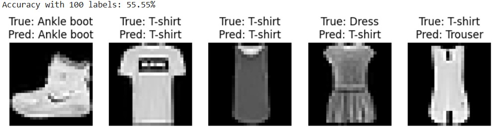
print(f"Accuracy with {n_labeled} labels: {accuracy:.2%}")

# 7. Class names for Fashion-MNIST
class_names = [
    "T-shirt", "Trouser", "Pullover", "Dress", "Coat",
    "Sandal", "Shirt", "Sneaker", "Bag", "Ankle boot"
]

# 8. Visualize some predictions
plt.figure(figsize=(10, 5))
for i in range(5):  # Show first 5 examples
    plt.subplot(1, 5, i+1)
    plt.imshow(X[i].reshape(28, 28), cmap='gray')
    true_name = class_names[y[i]]
    pred_name = class_names[model.predict([X[i]])[0]]
    plt.title(f"True: {true_name}\nPred: {pred_name}")
    plt.axis('off')
plt.show()

References

1. van Engelen, J. E., & Hoos, H. H. (2020). A survey on semi-supervised learning. Machine Learning, 109(2), 373–440. https://doi.org/10.1007/s10994-019-05855-6
2. IBM. (n.d.). Semi-supervised learning: What it is and why it matters. IBM Think. Retrieved August 2025, from https://www.ibm.com/think/topics/semi-supervised-learning