
Reinforcement Learning
- Reinforcement Learning (RL) is a machine learning method where an agent learns to make decisions through trial and error, which means rewards for correct actions and penalties for mistakes.
- The aim is to enforce correct actions to maximize future rewards.
- For example, when our child behaves well, we express appreciation, and when the child makes a mistake, we offer corrective feedback or reprimand. Over time, this helps the child gradually learn to distinguish between acceptable and unacceptable behavior.
Reinforcement Learning (RL) Process
A standard reinforcement learning framework (Markov Decision Process) can be illustrated using the following diagrammatic representation: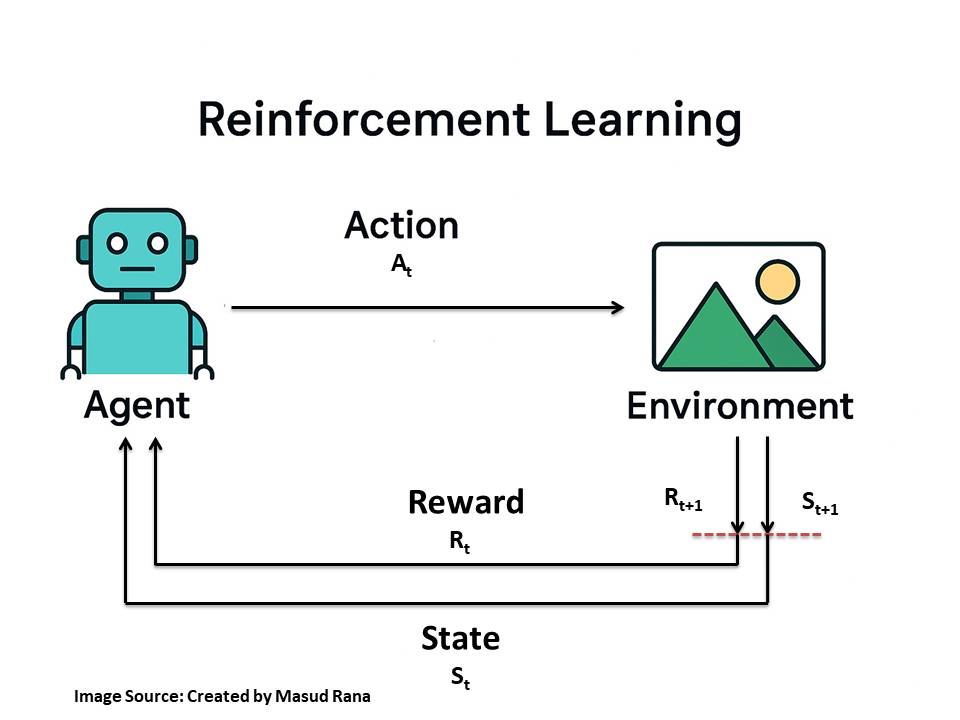
Key Components:
- Agent – The learner/decision-maker that chooses actions based on the current state St
- Environment – The external system that responds to the agent’s actions and provides feedback.
- State (Sₜ) – The current situation or observation the agent receives from the environment at time t.
- Action (Aₜ) – The move or decision the agent takes at time t to influence the environment.
- Reward (Rₜ) – The feedback signal from the environment indicating the success or failure of the action at time t.
The cycle works as flow:
- At time t, the environment sends the state (Sₜ) and reward (Rₜ) to the agent.
- The agent chooses an action (Aₜ).
- The environment processes that action, updates its situation, and produces the next state (Sₜ₊₁) and reward (Rₜ₊₁).
- The dotted line indicates the future state and reward (Sₜ₊₁, Rₜ₊₁). It represents the transition from the current step to the next step in time, showing that RL is a sequential process where each step influences the next.
How it works:
- Interaction: The agent observes the current state of the environment and selects an action based on its current understanding of the environment (policy π).
- Action Execution: The chosen action is performed, and the environment transitions to a new state (St+1).
- Feedback: The environment provides a reward signal to the agent, indicating the outcome of the action.
- Learning: The agent uses this reward (and potentially the new state) to update its understanding of the environment, i.e, update its value/Q-function and improve its decision-making strategy (policy π).
- Iteration: This process of interaction, feedback, and learning repeats, with the agent progressively refining its policy to maximize its cumulative reward over time (called return)
Types of Reinforcement Learning
Reinforcement learning (RL) has several approaches, but three foundational methods are under two types of Reinforcement Learning:
1. Model-Based RL
The agent builds a model of the environment to predict outcomes before acting.
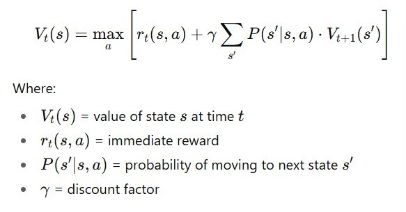
1.1 Dynamic Programming (DP)
- Breaks a big problem into smaller steps and uses a complete model of the environment to decide the best actions.
- Key Equation – Bellman Equation:
2. Model-Free RL
The agent learns from experience without knowing the full rules of the environment.
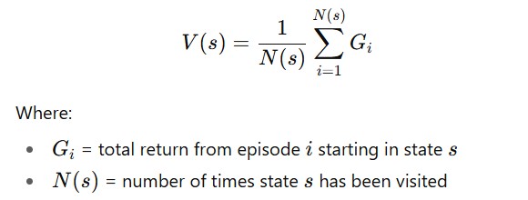
2.1 Monte Carlo (MC)
- Learns only from complete episodes of experience by averaging returns for each state–action pair.
- Key Equation – Value Function Estimate:
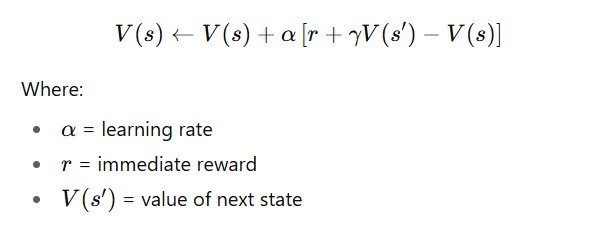
2.2 Temporal Difference (TD) Learning
- Learns from raw interaction but updates after every step without waiting for the episode to finish.
- Key Equation – TD Update Rule:
2.2.1 SARSA (State–Action–Reward–State–Action)
- It is on-policy Temporal Difference (TD) learning
- The agent learns the value of the policy it is following (including its exploration).
- Process:
- Start in state s, take action a.
- Receive reward r and move to next state s′.
- Choose the next action a′ based on the current policy.
- Update Q-value using:
Q(s,a)←Q(s,a)+α [ r+γQ(s′,a′)−Q(s,a)]
- Key Point: SARSA learns from the sequence (S, A, R, S’, A’), so it evaluates and improves the same policy it uses.
2.2.2 Q-Learning
- It is off-policy Temporal Difference (TD) learning
- The agent learns the optimal policy regardless of the actions it’s currently taking for exploration.
- Process:
- Start in state s, take action a.
- Receive reward r and move to next state s′.
- Look at the best possible next action a′ (max Q-value), even if the agent wouldn’t actually choose it during exploration.
- Update Q-value using:
Q(s,a)←Q(s,a)+ α [ r+γ max Q(s′,a′)−Q(s,a)]
- Key Point: Q-learning always learns towards the best possible policy (greedy with respect to Q-values), even if it explores randomly during learning.
Reinforcement Learning Methods
In Reinforcement Learning, online and offline learning are two main approaches to collecting data for policy training.
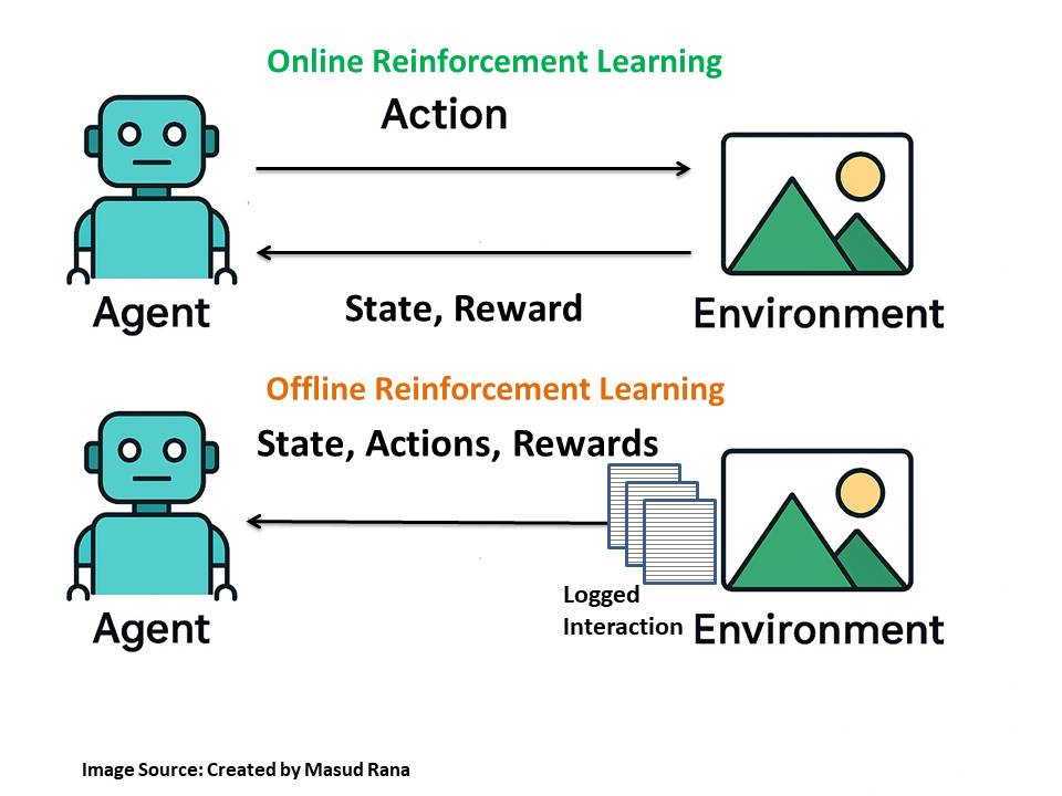
1. Online RL
- Definition: Agent learns by directly interacting with the environment.
- How it works: Takes an action → gets feedback (reward/penalty) → updates its policy → repeats.
- Example:
- A self-driving car learning to drive by actually driving on roads and adjusting in real-time to traffic, pedestrians, and road conditions.
- A robotic arm learning to stack boxes by trying, failing, and improving with each attempt.
2. Offline RL
- Definition: Agent learns from previously collected data without interacting with the environment during training.
- How it works: Uses logged data of states, actions, and rewards to train a policy without risking real-time mistakes.
- Example:
- A self-driving car is trained on millions of recorded hours of human driving data before being tested on the road.
- A recommendation system learning from past user interaction logs (e.g., Netflix recommendations trained from historical viewing data).
Applications of Reinforcement Learning (RL)
Reinforcement Learning (RL) is a powerful AI technique where an agent learns by interacting with its environment, receiving rewards for good actions and penalties for bad ones. Here are some key real-world applications:
1. Robotics
- Helps robots perform complex tasks like walking, grasping objects, or even driving.
- Uses deep learning to process sensory data (like cameras or sensors) and make decisions.
- Improves adaptability in changing environments, like self-driving cars.
2. Natural Language Processing (NLP) & Chatbots
- Enhances chatbot conversations by improving response quality.
- Uses Large Language Models (LLMs) to simulate real-world interactions.
- Helps in training AI for text-based decision-making (e.g., customer support bots).
3. Business, Marketing & Advertising
- Analyzes customer behavior to improve ads and promotions.
- Helps companies create better sales strategies by predicting trends.
- Used by big corporations to maximize profits (but can be expensive).
4. Gaming
- Powers advanced AI in games (e.g., chess, Go, video games).
- Algorithms like AlphaGo and AlphaZero beat human champions.
- Enhances game realism with adaptive AI opponents.
5. Recommendation Systems
- Used by Netflix, Spotify, and news apps to suggest content.
- Learns from user preferences to recommend movies, songs, or articles.
- Improves over time based on user interactions.
6. Science & Research
- Helps in studying chemical reactions and molecular structures.
- Used in physics and chemistry to simulate experiments.
- Deep RL models (like LSTM) improve accuracy in scientific predictions.
Python Implementation of Reinforcement Learning
# Importing necessary libraries
import numpy as np
import pandas as pd
import random
import matplotlib.pyplot as plt
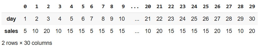
# Creating the fashion sales dataset
data = pd.DataFrame({
"day": range(1, 31),
"sales": np.random.choice([5, 10, 15, 20], size=30, p=[0.2, 0.4, 0.3, 0.1])
})
# Showing dataset in horizontal way for better visibility
data.T
# Reinforcement Learning environment setup

states = ["low", "medium", "high"]
actions = ["restock", "do_nothing"]

Q = pd.DataFrame(0, index=states, columns=actions)
Q
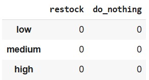
- States:
- low → inventory less than 10
- medium → inventory between 10 and 19
- high → inventory 20 or above
- Actions: The agent can either restock or do nothing.
- Q-table: A table where each (state, action) pair has a Q-value (expected reward). Initially, all are set to 0.
# RL parameters
alpha = 0.1      # learning rate (how much we update)
gamma = 0.9      # discount factor (future reward importance)
epsilon = 0.2    # exploration rate (chance to try random actions)
- α (alpha) → small update steps to avoid overfitting to recent experiences.
- γ (gamma) → high value = agent cares about future rewards almost as much as immediate rewards.
- ε (epsilon) → 20% of the time the agent explores randomly.
# State function- Inventory thresholds

def get_state(inventory):
    if inventory < 10:
        return "low"
    elif inventory < 20:
        return "medium"
    else:
        return "high"
- Converts numeric inventory into a category (low, medium, high).
# Reward function

def get_reward(inventory, sales):
    if sales > inventory:
        return -10  # stockout → lose sales, unhappy customers
    elif inventory - sales > 15:
        return -5   # overstock → too much unsold stock
    else:
        return 10   # just right
- Negative reward for:
- Stockouts (lost customers)
- Overstock (wasted storage money)
- Positive reward when inventory matches demand well.
# Store Q-values over time
q_history = {state: {action: [] for action in actions} for state in states}

# Q-learning loop

inventory = 15
for episode in range(200):  # train for 200 iterations
    for _, row in data.iterrows():
        state = get_state(inventory)

        # Choose action (epsilon-greedy)
        if random.uniform(0, 1) < epsilon:
            action = random.choice(actions)   # explore
        else:
            action = Q.loc[state].idxmax()    # exploit

        # Apply action
        if action == "restock":
            inventory += 10

        sales = row["sales"]
        reward = get_reward(inventory, sales)
        inventory -= sales
        inventory = max(0, inventory)  # no negative stock

        # New state after sales
        next_state = get_state(inventory)

        # Q-learning update (Bellman equation)
        Q.loc[state, action] += alpha * (
            reward + gamma * Q.loc[next_state].max() - Q.loc[state, action]
        )
        # Record Q-values
        for s in states:
            for a in actions:
                q_history[s][a].append(Q.loc[s, a])
- State is determined from the current inventory.
- Action is chosen:
- Random (explore) 20% of the time.
- Best known action (exploit) otherwise.
- Action effect:
- Restocking adds +10 units to inventory.
- Sales happen (taken from the dataset).
- Reward is calculated based on how well we met demand.
- Inventory updates after sales.
- Q-table updated using the Bellman update rule:
- Immediate reward + best possible future reward.
# Result

print("\nTrained Q-table:\n",Q)
Trained Q-table:
           restock  do_nothing
low     59.260479   42.199421
medium  62.090124   34.279440
high     1.429011    0.000000
After training, the Q-table tells you which action gives higher expected rewards in each inventory state.
For example:
- If low inventory, → likely restock will have a high Q-value.
- If high inventory → likely do nothing will have a high Q-value.
#Plot Q-values over time ---

plt.figure(figsize=(12, 6))
for s in states:
    for a in actions:
        plt.plot(q_history[s][a], label=f"{s} - {a}")
plt.xlabel("Training Steps")
plt.ylabel("Q-value")
plt.title("Q-values over Time for Fashion Inventory RL Agent")
plt.legend()
plt.grid(True)
plt.show()
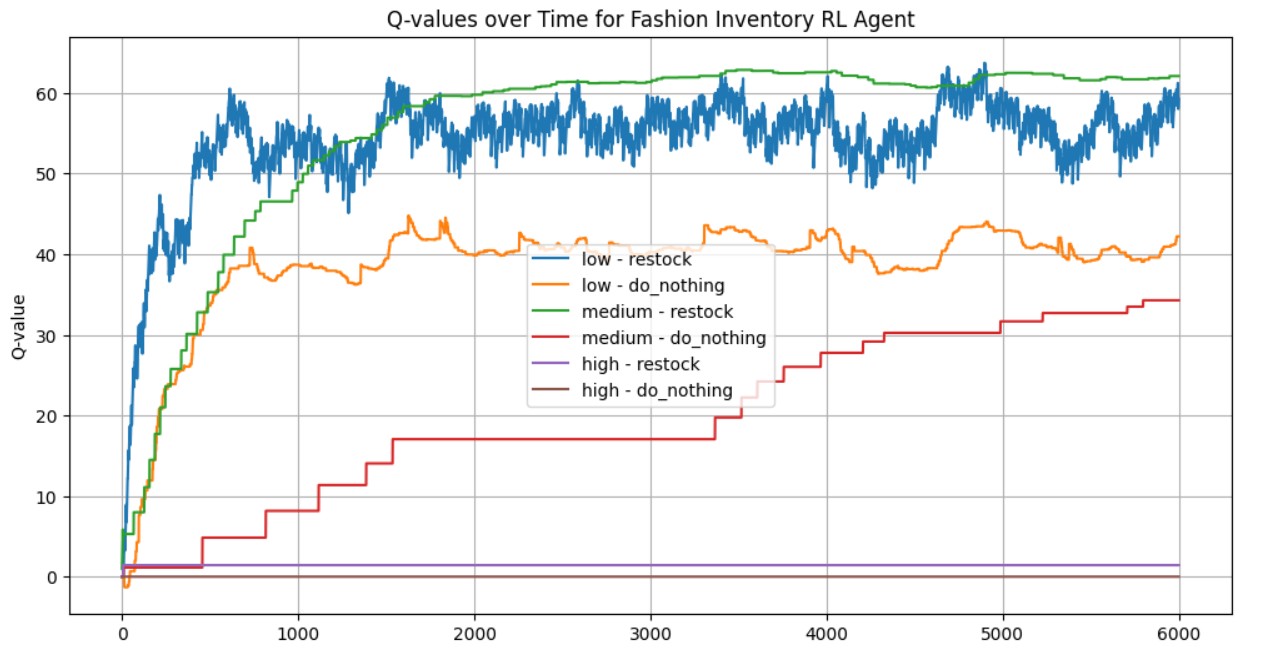
Observations:
1. Low inventory:
- Restock (blue): Starts low, quickly rises, and stabilizes at a high value (~55–60), indicating that restocking when inventory is low is learned as a highly rewarding action.
- Do nothing (orange): Also rises initially but stabilizes much lower (~40), suggesting it’s less optimal.
2. Medium inventory:
- Restock (green): Gradually increases and stabilizes at a high Q-value (~60), showing that restocking is still considered valuable here.
- Do nothing (red): Increases slowly and stays much lower (~30), indicating it’s less favorable.
3 .High inventory:
- Restock (purple): Flat and near zero, meaning the agent sees almost no benefit in restocking when inventory is already high.
- Do nothing (brown): Slight increase from zero, suggesting a small benefit but still not a high reward.
Interpretation:
- The RL agent has learned sensible behavior:
- Restock when inventory is low or medium → high Q-values.
- Avoid restocking when inventory is high → low Q-values.
- The separation between Q-value lines shows clear policy preference formation.
- Early in training, Q-values fluctuate as the agent explores; later, they stabilize as the policy converges.
ChatGPT said:
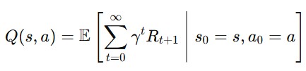
Where:
- Rt+1 = reward after taking action at time t
- γ = discount factor (how much we value future rewards)
- The expectation E is over possible outcomes (since the environment may be stochastic).
Reference
- GeeksforGeeks. “What is Reinforcement Learning?” Available at: https://www.geeksforgeeks.org/machine-learning/what-is-reinforcement-learning/
- IBM. “Reinforcement Learning.” Available at: https://www.ibm.com/think/topics/reinforcement-learning
- TechVidvan. “Reinforcement Learning.” Available at: https://techvidvan.com/tutorials/reinforcement-learning/
- Al-Dujaili, A., Kearnes, S., & Gomes, C. P. (2022). “Reinforcement Learning: Fundamentals, Methods, and Applications.” Available at: https://arxiv.org/pdf/2209.14940
