
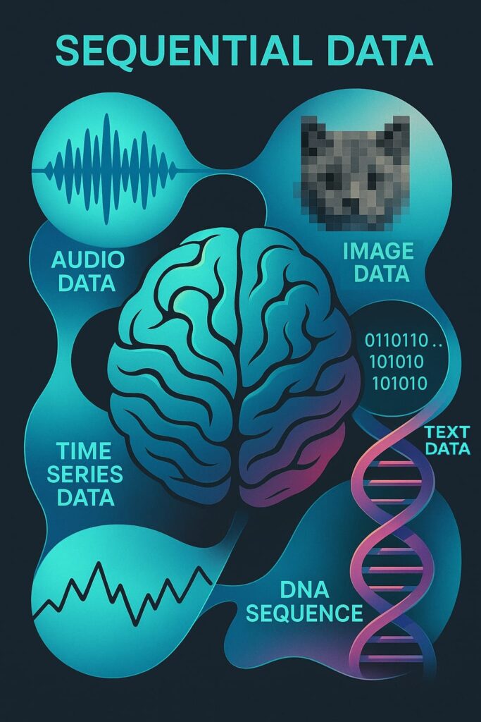
Sequential Data:
- Sequential Data are such data where the order of elements is matter
- Elements are dependent on the previous ones
- Example of Sequential Data:
- Time Series Data: Data points collected or recorded at specific time intervals, such as stock prices, temperature readings, or heart rate monitoring.
- Text Data: Sequences of words or characters, where the meaning of a word can depend on the words that come before it.
- Speech Data: Audio signals that vary over time, where the sequence of sounds forms words and sentences.
- Video Data: A sequence of frames (images) that, when played in order, create a moving picture.
- DNA Sequences: Biological sequences where the order of nucleotides is crucial for the genetic information they carry.
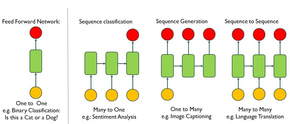
Applications of Sequence Modelling:
While basic neural network (Vanilla Neural Network) gives single output from single input as in image below from left first one which is simple neural network, Sequence model can do below 3 operations :
- Many input to one output : Process the many words in the individual sentences & produce a output. For example, sentiment analysis where sentences could have positive or negative reviews.
- One input to many output : Taking one image & produce caption of the image which is sentence of many words. For example, image captioning.
- Many input to many output : Taking a sentence with many words & produce another sentence with many words. For example, Translation from one language to another language.
The term “Vanilla Neural Network” means the most basic neural network – also known as a Feedforward Neural Network (FNN) or Multilayer Perceptron (MLP).
Neurons with Recurrence:
We will now see the transition from a simple, memoryless model (vanilla NN) to a dynamic model (RNN) that captures time dependencies by recycling hidden states across time.
Start with a Vanilla Neural Network
- Imagine a basic feedforward neural network (vanilla NN) where input flows from left to right (or bottom to top if rotated).
Apply it to Sequential Data
- Sequential data has multiple time steps (e.g., t0, t1, t2, etc.).
- Initially, we might think of running the same neural network on each time step independently (treating each as an isolated input-output pair).
Identify the Problem
- When we process each time step independently, the model ignores the relationship between time steps.
- In sequential data (like text, stock prices, speech), the current prediction depends on previous data. Ignoring past time steps leads to poor modeling of the sequence.
Introduce the Concept of Memory
- To address this, you need a way to “remember” past information.
- The solution is to pass information forward in time within the network using an internal state.
Define an Internal State (hₜ)
- Introduce a hidden/internal state variable h(t).
- h(t) acts like a memory cell that holds information about past computations (e.g., what happened at t0 and t1 when computing output at t2).
New Output Dependency
- Now the output ŷ(t) at time step t depends on:
- The current input x(t)
- The internal state h(t-1) passed from the previous time step.
Formula: Yt = f ( Xt , ht-1 )
- Now the output ŷ(t) at time step t depends on:
Recurrence Relation
- This recursive dependency (passing h(t) forward in time) creates a recurrence relation, meaning the computation at time t is influenced by past computations.
Visualization
- Unrolled View: Time steps are laid out as a sequence, and h(t) connects each time step like a chain.(reader right of end of the video)
- Loop View: Represented as a looped diagram showing the hidden state feeding back into itself across time steps.(reader left of end of video)
Recurrent Neural Networks
- This architecture forms the foundation of Recurrent Neural Networks (RNNs).
- Unlike a vanilla NN, an RNN maintains internal memory and is capable of capturing temporal dependencies within sequential data.
Please click on video to see visualization of above explanation
Definition of RNNs:
- An RNN (Recurrent Neural Network) is a type of neural network that is specifically designed to handle sequential data.
- Unlike traditional feedforward neural networks, which process inputs independently, an RNN introduces loops within the network.
- These loops enable information to persist, meaning the output of a neuron at a one-time step is fed back into the network as input at the next time step.
This feedback mechanism creates a form of short-term memory—allowing the network to retain contextual information from previous inputs, which is critical when dealing with time-dependent data, text data, etc.
RNN Architecture Overview:
At its core, an RNN processes input sequences step-by-step, maintaining a hidden state vector that captures information about previous elements in the sequence.
Each time step has:
- Input (xₜ): The data at time step t.
- Hidden State (hₜ): The “memory” carried from one-time step to the next.
- Output (yₜ): The prediction or processed value at time t.
The hidden state is updated using the formula:
hₜ = fw(xₜ , hₜ₋₁)
Here,
hₜ = New state
xₜ = Input vector
hₜ₋₁ = Old State
fw = Activation Function
Also we can write as, hₜ = f(Wₓ * xₜ + Wₕ * hₜ₋₁)
Where Wₓ and Wₕ are learned weight matrices, and f is an activation function like tanh or ReLU.
For a simple RNN we can write as below:

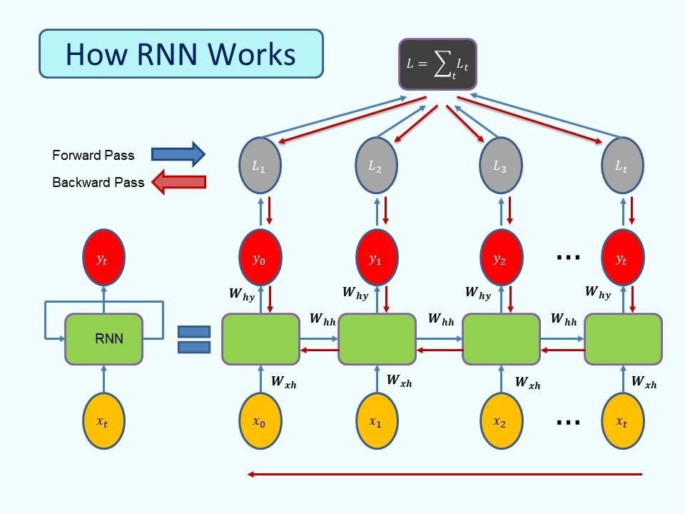
How RNNs Work (Unfolding RNNs)
To better understand Recurrent Neural Networks (RNNs), let’s unfold the network over time and walk through the step-by-step process.
01. Input Sequence Preparation
- Input sequence:x1, x2, ….. , xT
- May include preprocessing like tokenization (for text), normalization (for time series), or embedding (for categorical inputs).
02. Weight Matrices in an RNN
RNNs use three key weight matrices that are shared and reused at every time step in the sequence:
Wxh : Transforms the input vector xt into the hidden state
Whh : Updates the hidden state by combining it with the previous hidden state ht−1
Why: Maps the hidden state to the output prediction (ŷ).
These weights remain the same throughout the entire sequence, allowing the RNN to generalize across time.
03. The Forward Pass (Unfolding Through Time)
At each time step t , the RNN performs the following operations:
Hidden State Update:
ht=tanh(Wxhxt+Whhht−1+bh
Output Prediction:
ŷ =softmax(Whyht+by)
These steps are repeated across time steps: t=0→1→2→⋯→T
This sequence of computations is called the forward pass.
04. Loss Calculation
Like other neural networks, RNNs require a loss function to evaluate how far the predicted output ŷtis from the true label yt
At each time step, compute the loss between ŷt and yt
The total loss across all time steps is:
Total Loss = ∑ Loss(ŷt ,yt)
This total loss guides the training process.
05. Backpropagation Through Time (BPTT)
It is the process of training an RNN by computing gradients over multiple time steps. :
- After the forward pass, compute the total loss.
- Then, propagate the gradients backward through each time step, from T→T−1→⋯→0
- Gradients are used to update:
- Input weights Wxh
- Hidden weights Whh
- Output weights Why
Because the hidden state depends on previous time steps, the gradients also flow through all previous hidden states, making training more complex than in feedforward networks.
06. Weight Updates
- Apply gradient descent (or any optimizer like Adam or RMSProp): W:=W−η⋅∇WL
| Symbol | Meaning |
|---|---|
| W | A weight matrix |
| := | This means we are updating or replacing the old value |
| η | The learning rate — a small positive number (like 0.01 or 0.001) |
| ∇WL | The gradient (∇ = “nabla”) of the loss L with respect to the weight W — this tells us how the loss changes if we change W slightly |
Problem with RNNs
RNNs can struggle with long sequences due to the vanishing or exploding gradient problem, which makes it hard for the network to learn long-term dependencies.
1. Vanishing Gradient Problem
- During backpropagation, we multiply many small gradient values over time.
- These values can become very, very small (close to zero).
- As a result:
- Earlier layers (older time steps) get almost no update.
- The model forgets long-term patterns.
- It can’t learn long-term dependencies (like remembering something from 10 steps ago).
2. Exploding Gradient Problem
- Sometimes, instead of shrinking, the gradients grow too large during backpropagation.
- This causes:
- Huge weight updates.
- The model becomes unstable.
- The loss might become NaN (Not a Number).
Both problems make it hard for RNNs to learn properly, especially with long sequences like:
- Sentences in natural language processing
- Long time-series data
Advanced variants like LSTM and GRU address this issue by using gates to control the flow of data. We will discuss LSTM and GRU in the next chapter
Sequence Modeling: Design Criteria
Sequence models need to do-
- Variable-length handling:
- Sequences can be short or long (e.g., one sentence vs. a full paragraph).
- Track long-term dependencies:
- Understand relationships far apart in the sequence (e.g., the subject at the start of a sentence and its verb much later).
- Maintain order:
- Sequences are ordered. “The cat sat” ≠ “Sat the cat”.
- Share parameters:
- The model uses the same weights at every time step, making it efficient and generalizable.
Why RNNs fit the above design criteria:
- RNNs loop back on themselves to process each input step-by-step, maintaining memory (hidden state).
- This looping structure allows them to:
- Handle any length.
- Remember past steps (though not always perfectly).
- Keep track of sequence order.
Sequence Modelling Problem: Predict the Next Word
Let’s Demonstrate a sequence modeling problem step-by-step where the goal is to predict the next word in a sentence.
Given the sentence “The cat is sitting on the” and our goal is to predict the next word.
- Task:
- Input: A sequence of words (e.g., “The cat is sitting on the”).
- Output: The most likely next word (e.g., “mat”, “floor”, “sofa”, etc.).
- Type of Model: Sequence-to-One (sequence in → single prediction out).
- Encoding language for a Neural Network:
- Vocabulary: Corpus of words with all possible words we could encounter
- Word Indexing: taking individual words from vocabulary & map them into index number
- the → 1
- cat → 2
- … → …
- mat → N
- Embedding: Transform indexes into a vector of fixed size by One Hot Encoding
Please click on video to see visualization of above explanation:
What is a Semantic Space?
- A semantic space is a vector space which encodes ‘meanings’ of words
- Words embedded in vectors that are similar in meaning or used in similar contexts are placed closer together in this space.
- Think of it like a map where:
- Paris and London are near each other.
- Paris and Banana are very far apart.

Python Implementation for RNN(Prediction Fashion Product Description)
# Import Necessary Libraries
import numpy as np
import pandas as pd
import matplotlib.pyplot as plt
import tensorflow as tf
from tensorflow.keras.models import Sequential
from tensorflow.keras.layers import Embedding, SimpleRNN, Dense
from tensorflow.keras.preprocessing.text import Tokenizer
from tensorflow.keras.preprocessing.sequence import pad_sequences
from sklearn.model_selection import train_test_split
# Step 1: Load fashion industry dataset
df = pd.read_csv('/content/fashion_descriptions.csv')
fashion_descriptions = df['description'].tolist()
# Step 2: Preprocess the text data
tokenizer = Tokenizer()
tokenizer.fit_on_texts(fashion_descriptions)
total_words = len(tokenizer.word_index) + 1
# Create input sequences
input_sequences = []
for line in fashion_descriptions:
token_list = tokenizer.texts_to_sequences([line])[0]
for i in range(1, len(token_list)):
n_gram_sequence = token_list[:i+1]
input_sequences.append(n_gram_sequence)
# Pad sequences
max_sequence_len = max([len(x) for x in input_sequences])
input_sequences = pad_sequences(input_sequences, maxlen=max_sequence_len, padding='pre')
# Create predictors and label
X = input_sequences[:, :-1]
y = input_sequences[:, -1]
# Convert y to one-hot encoding
y = tf.keras.utils.to_categorical(y, num_classes=total_words)
# Split into train and validation sets
X_train, X_val, y_train, y_val = train_test_split(X, y, test_size=0.2, random_state=42)
print("\nInput sequence shape:", X.shape)
print("Training data shape:", X_train.shape)
print("Validation data shape:", X_val.shape)
print("Output shape:", y.shape)
# Step 3: Build the RNN model
model = Sequential([
Embedding(total_words, 64, input_length=max_sequence_len-1),
SimpleRNN(100, return_sequences=True),
SimpleRNN(100),
Dense(total_words, activation='softmax')
])
model.compile(loss='categorical_crossentropy', optimizer='adam', metrics=['accuracy'])
print("\nModel summary:")
model.summary()
# Step 4: Train the model with validation
history = model.fit(
X_train, y_train,
validation_data=(X_val, y_val),
epochs=50,
batch_size=128,
verbose=1
)
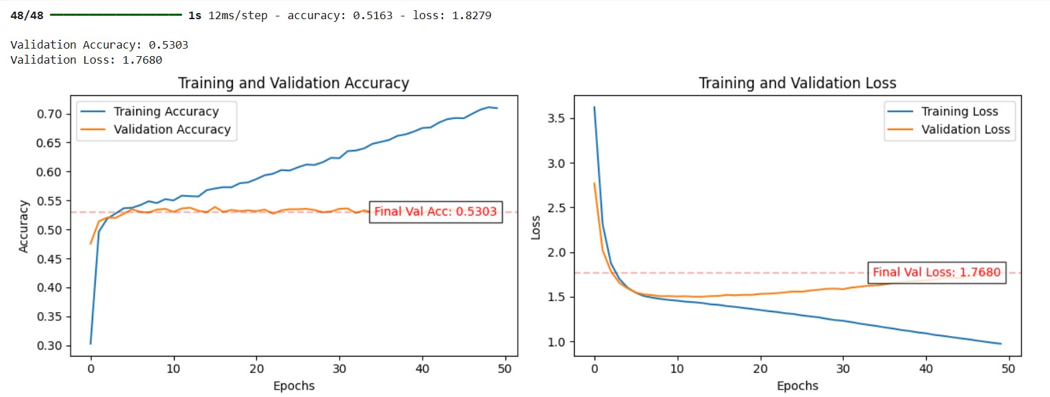
# Step 5: Model Evaluation with Scores on Plots
def plot_training_history(history, val_loss, val_acc):
plt.figure(figsize=(12, 4))
# Plot accuracy
plt.subplot(1, 2, 1)
plt.plot(history.history['accuracy'], label='Training Accuracy')
plt.plot(history.history['val_accuracy'], label='Validation Accuracy')
# Add final validation accuracy annotation
plt.axhline(y=val_acc, color='r', linestyle='--', alpha=0.3)
plt.text(len(history.history['accuracy'])-1, val_acc,
f'Final Val Acc: {val_acc:.4f}',
ha='right', va='center', color='red',
bbox=dict(facecolor='white', alpha=0.8))
plt.title('Training and Validation Accuracy')
plt.xlabel('Epochs')
plt.ylabel('Accuracy')
plt.legend()
# Plot loss
plt.subplot(1, 2, 2)
plt.plot(history.history['loss'], label='Training Loss')
plt.plot(history.history['val_loss'], label='Validation Loss')
# Add final validation loss annotation
plt.axhline(y=val_loss, color='r', linestyle='--', alpha=0.3)
plt.text(len(history.history['loss'])-1, val_loss,
f'Final Val Loss: {val_loss:.4f}',
ha='right', va='center', color='red',
bbox=dict(facecolor='white', alpha=0.8))
plt.title('Training and Validation Loss')
plt.xlabel('Epochs')
plt.ylabel('Loss')
plt.legend()
plt.savefig('Accuracy_Loss.png')
plt.tight_layout()
plt.show()
# Evaluate on validation set
val_loss, val_acc = model.evaluate(X_val, y_val, verbose=1)
print(f"\nValidation Accuracy: {val_acc:.4f}")
print(f"Validation Loss: {val_loss:.4f}")
# Plot with scores included
plot_training_history(history, val_loss, val_acc)
# Generate sample predictions

def generate_text(seed_text, next_words, model, tokenizer, max_sequence_len):
    for _ in range(next_words):
        token_list = tokenizer.texts_to_sequences([seed_text])[0]
        token_list = pad_sequences([token_list], maxlen=max_sequence_len-1, padding='pre')
        predicted_probs = model.predict(token_list, verbose=0)
        predicted_index = np.argmax(predicted_probs, axis=-1)[0]

        output_word = ""
        for word, index in tokenizer.word_index.items():
            if index == predicted_index:
                output_word = word
                break

        seed_text += " " + output_word
    return seed_text

print("\nGenerate fashion descriptions:")
print(generate_text(input(), 10, model, tokenizer, max_sequence_len))
Output:
Generate fashion descriptions:
elegant dress
elegant dress spandex sweatshirt is made of leather in beige color with
