Random Forest:
- A Random Forest is a supervised machine learning algorithm that builds upon the foundation of decision trees.
- It is commonly used to solve both classification and regression problems.
- Random Forest employs an ensemble learning technique, where multiple decision trees are constructed and combined to improve predictive performance and reduce overfitting.
- Each tree in the forest makes its own prediction, and the final output is determined by aggregating those predictions – using the majority vote for classification or the average for regression tasks.
- By increasing the number of trees in the forest, the model typically gains greater accuracy and robustness, as it minimizes the impact of any single poorly performing tree.
How Random Forest Works (ensemble learning):
1. Bootstrap Sampling
- During training, each tree in a Random Forest is built using a random sample of the dataset.
- This sampling is done with replacement, a process known as bootstrapping.
- As a result, some data points may appear multiple times in the same sample, while others may be excluded entirely from that tree’s training data.
2. Aggregation
Once all trees are trained, the Random Forest makes predictions through a process called aggregation:
For regression tasks, it returns the average of the predictions from all trees.
For classification tasks, it uses majority voting to decide the final class label.
This combination of bootstrap sampling and aggregation makes Random Forests robust, accurate, and less prone to overfitting compared to individual decision trees.
Pros:
High accuracy and robustness due to ensemble learning (multiple trees).
Handles both classification and regression effectively.
Cons:
- Hard to interpret compared to a single decision tree (black box model).
Python Implementation for Random Forest for Classification Task:
# Step 1: Import required libraries
from sklearn.ensemble import RandomForestClassifier
from sklearn.metrics import accuracy_score, classification_report
from tensorflow.keras.datasets import fashion_mnist
import matplotlib.pyplot as plt
# Step 2: Load the fashion dataset
(X_train, y_train), (X_test, y_test) = fashion_mnist.load_data()
# Step 3: Preprocess data - Flatten the 28x28 images to 784 features
X_train_flat = X_train.reshape(-1, 28 * 28) / 255.0
X_test_flat = X_test.reshape(-1, 28 * 28) / 255.0
# Step 4: Initialize and train the Random Forest model
rf_model = RandomForestClassifier(n_estimators=100, max_depth=20, random_state=42)
rf_model.fit(X_train_flat, y_train)
# Step 5: Predict and evaluate
y_pred_rf = rf_model.predict(X_test_flat)
Random_Forest_Accuracy = accuracy_score(y_test, y_pred_rf)
# Step 6: Visualize predictions
fashion_labels = ['T-shirt/top', 'Trouser', 'Pullover', 'Dress', 'Coat',
'Sandal', 'Shirt', 'Sneaker', 'Bag', 'Ankle boot']
plt.figure(figsize=(10, 6))
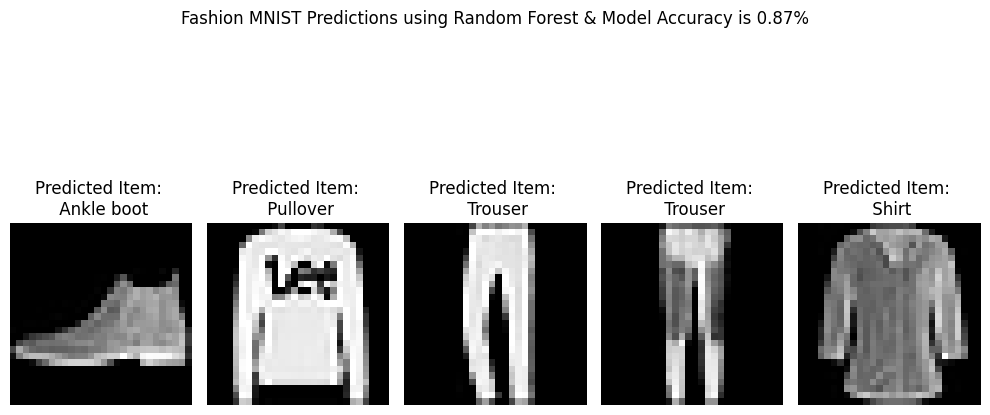
for i in range(5):
plt.subplot(1, 5, i+1)
plt.imshow(X_test[i], cmap='gray')
plt.title(f"Predicted Item: \n {fashion_labels[y_pred_rf[i]]}")
plt.axis('off')
plt.suptitle(f"Fashion MNIST Predictions using Random Forest & Model Accuracy is {Random_Forest_Accuracy:.2f}%")
plt.tight_layout()
plt.show()
Python Implementation for Random Forest for Regression Task:
# Step 1: Import necessary libraries
import pandas as pd
import numpy as np
from sklearn.ensemble import RandomForestRegressor
from sklearn.model_selection import train_test_split
from sklearn.metrics import mean_squared_error, r2_score
import matplotlib.pyplot as plt
# Step 2: Loading Dataset
data = pd.read_csv('/content/Clothing_price')
# Step 3: Train/Test Split
X = data.drop('price', axis=1)
y = data['price']
X_train, X_test, y_train, y_test = train_test_split(X, y, test_size=0.2, random_state=42)
# Step 4: Train Decision Tree Regressor
rf_model = RandomForestRegressor(n_estimators=100, max_depth=10, random_state=42)
rf_model.fit(X_train, y_train)
# Step 4: Predictions & Evaluation
y_pred_rf = rf_model.predict(X_test)
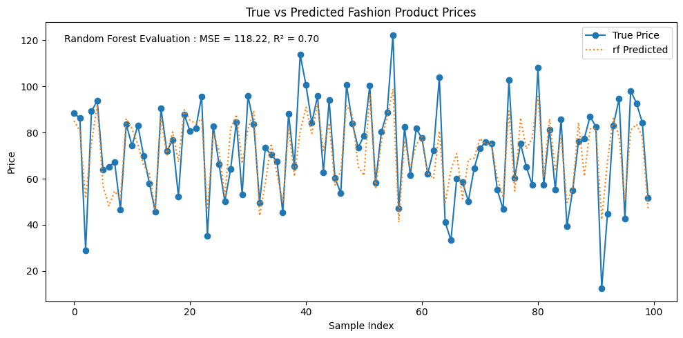
plt.figure(figsize=(10, 5))
plt.plot(y_test.values, label='True Price', marker='o')
plt.plot(y_pred_rf, label='rf Predicted', linestyle=':')
r2_dt = r2_score(y_test, y_pred_rf)
mse_dt = mean_squared_error(y_test, y_pred_rf)
plt.annotate(f"Random Forest Evaluation : MSE = {mse_dt:.2f}, R² = {r2_dt:.2f}",
xy=(0.03, 0.93),xycoords='axes fraction')
plt.legend()
plt.title("True vs Predicted Fashion Product Prices")
plt.xlabel("Sample Index")
plt.ylabel("Price")
plt.tight_layout()
plt.show()