Long Short-Term Memory (LSTM) Networks

LSTM

• LSTM stands for Long Short-Term Memory, a special type of Recurrent Neural Network (RNN) capable of learning long-term dependencies in sequential data, such as text, time series, speech, or any ordered data.

Why Do We Need LSTM?

In many real-world problems, especially involving sequences like:

• Predicting stock prices 
• Understanding language
• Music generation 
• Forecasting weather 
  …we need models that remember past information to make better predictions.

Imagine reading a sentence:

“The girl who loved books went to the library.”

To understand “went to the library,” the model needs to remember that it’s “the girl” who is doing the action.

• As we know, basic RNNs forget long-term dependencies due to a problem known as the vanishing gradient. This makes them poor at remembering things from earlier in a long sequence.
• LSTMs solve this problem using a gating mechanism that regulates the flow of information.

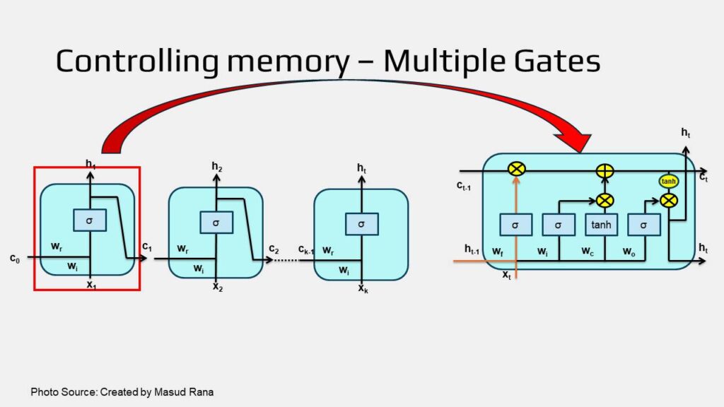
Controlling Memory by Multiple Gates

• All recurrent neural networks (RNNs) are made up of a sequence of repeating modules, which pass information from one step to the next.
• In a standard RNN, each of these modules has a very simple design, usually consisting of just one layer.

However,

• Long Short-Term Memory networks (LSTMs) also follow this chain-like structure, but each repeating module is more complex.
• Instead of using a single layer, an LSTM module contains four specialized layers that work together uniquely to better manage and control the flow of information over time (As in the image below).

The Intuition Behind LSTM

• At the core of an LSTM network is the cell state, which is represented by the horizontal line running across the top of the diagram.
• We can think of the cell state as a conveyor belt that carries information across the sequence.
• It moves through the network with minimal changes, allowing important information to flow forward easily.

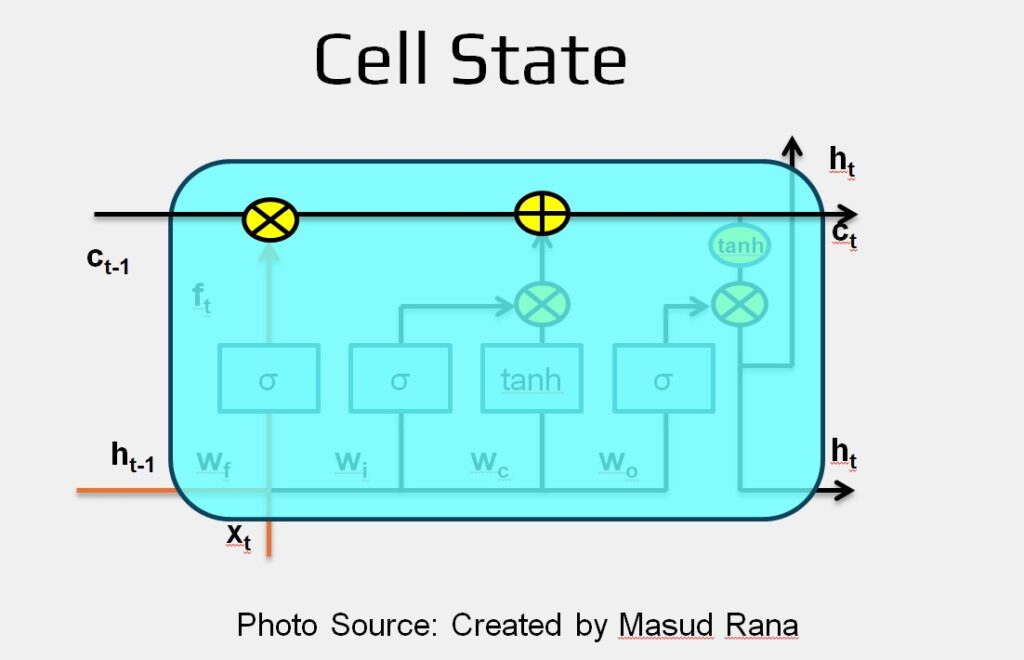
• However, the LSTM can update this cell state by either removing or adding information. This process is carefully managed by special components called gates.

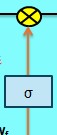
Gates are mechanisms that control the flow of information. Each gate consists of two parts:

• A sigmoid layer, which outputs values between 0 and 1 to decide how much information should pass through.
• A pointwise multiplication that applies this decision to the data.
  • A value close to 0 means “block everything.”
  • A value close to 1 means “let everything through.”

LSTMs use three gates: the forget gate, input gate, and output gate — to protect and manage the cell state, allowing the model to learn and remember important patterns over time.

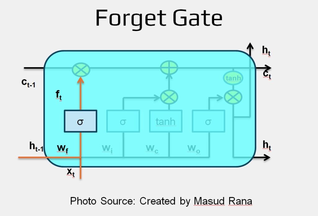
Forget Gate

The first step in an LSTM is to decide what information should be removed from the cell state. This is done by a special component called the forget gate, which uses a sigmoid activation layer.

This gate takes in two inputs:

• Previous hidden state h_t−1​
• Current input x
  

It then produces a value between 0 and 1 for each part of the previous cell state C_t−1​:

• A value close to 1 means “keep this information completely.”
• A value close to 0 means “forget this completely.”

Forget Gate Equation:  f_t = σ ( W _f ⋅ [ h _t−1 , x_t ] + b_f )

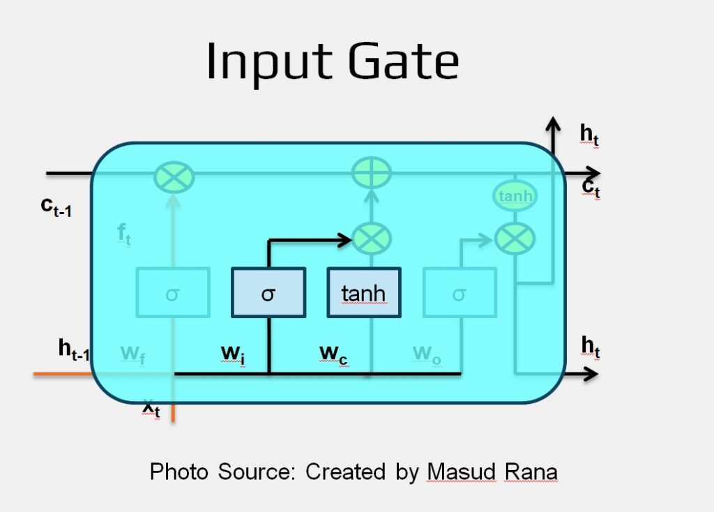
Input Gate

The next step in the LSTM process is to decide what new information should be added to the cell state. This step is made up of two parts:

1. A sigmoid layer called the input gate determines which parts of the new information are important enough to update the cell state. 

   Input Equation i_t  = σ (W_i * [ h_t−1 , x_t ] + b_i )

2. A tanh layer creates a vector of new candidate values (C~_t​) that represent potential information to be stored.

   Candidate Value Equation: C_t~ = tanh (w_c * [ h_t-1 , x_t ] + b_c )

In the following step, these two outputs will be combined to update the cell state.

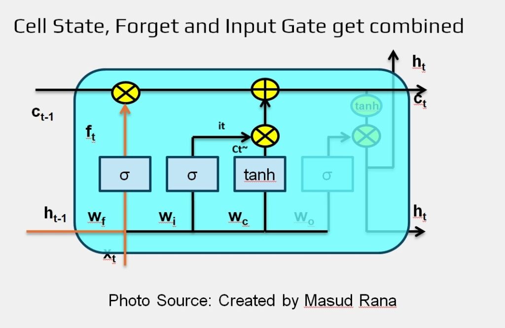
Combine Cell State, Forget, Input Gate

Now it’s time to update the cell state from the old version C_t-1​ to the new version C_t​. The earlier steps have already determined what to forget and what to add—this step simply applies those decisions.

• First, we multiply the old cell state by the forget gate output f_t​. This step removes the parts of the memory we decided were no longer useful.

• Then, we add the result of the input gate i_t​ multiplied by the candidate values C_t~. This means we’re adding new information, but only the parts that the input gate allowed through.

Combined Equation: C_t = f_t * C_t-1 + i_t * C_t~

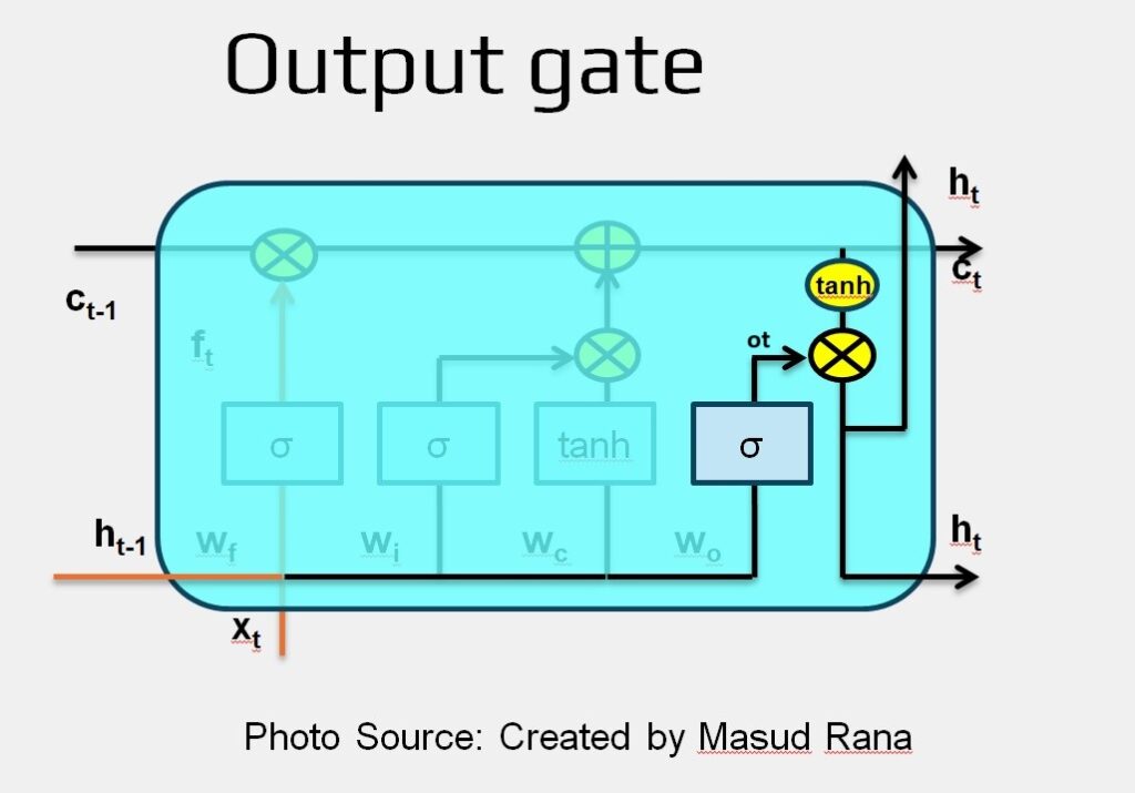
Output Gate

The final step in the LSTM process is to decide what information to output. This output is based on the updated cell state, but it’s not a direct copy—it goes through a filtering process.

1. First, a sigmoid layer (called the output gate) determines which parts of the cell state should influence the output.
2. Then, the cell state is passed through a tanh function, which scales its values to be between -1 and 1.
3. Finally, we multiply the tanh-transformed cell state by the output gate’s result, so that only the selected parts are included in the final output.

Output Equation : o_t = σ (W_o * [ h_t−1 , x_t ] + b_o )

New Hidden State Equation: h_t = o_t * tanh(C_t)

Python Implementation of LSTM (Fashion Product Description Generator)

# Import Necessary Libraries
import numpy as np
import pandas as pd
import matplotlib.pyplot as plt

import tensorflow as tf
from tensorflow.keras.models import Sequential
from tensorflow.keras.layers import Embedding, LSTM, Dense
from tensorflow.keras.preprocessing.text import Tokenizer
from tensorflow.keras.preprocessing.sequence import pad_sequences

from sklearn.model_selection import train_test_split

# Step 1: Load fashion dataset
df = pd.read_csv('/content/fashion_descriptions.csv')
fashion_descriptions = df['description'].astype(str).tolist()

# Step 2: Preprocess the text data
tokenizer = Tokenizer()
tokenizer.fit_on_texts(fashion_descriptions)
total_words = len(tokenizer.word_index) + 1

# Create input sequences using n-gram method
input_sequences = []
for line in fashion_descriptions:
    token_list = tokenizer.texts_to_sequences([line])[0]
    for i in range(1, len(token_list)):
        n_gram_sequence = token_list[:i+1]
        input_sequences.append(n_gram_sequence)

# Pad sequences
max_sequence_len = max([len(x) for x in input_sequences])
input_sequences = pad_sequences(input_sequences, maxlen=max_sequence_len, padding='pre')

# Create predictors and label
X = input_sequences[:, :-1]
y = input_sequences[:, -1]
y = tf.keras.utils.to_categorical(y, num_classes=total_words)

# Train-validation split
X_train, X_val, y_train, y_val = train_test_split(X, y, test_size=0.2, random_state=42)

# Step 3: Build the LSTM model
model = Sequential([
    Embedding(total_words, 64, input_length=max_sequence_len-1),
    LSTM(128, return_sequences=True),
    LSTM(64),
    Dense(64, activation='relu'),
    Dense(total_words, activation='softmax')
])

model.compile(loss='categorical_crossentropy', optimizer='adam', metrics=['accuracy'])
model.summary()

# Step 4: Train the model
history = model.fit(
    X_train, y_train,
    validation_data=(X_val, y_val),
    epochs=80,
    batch_size=128,
    verbose=1
)

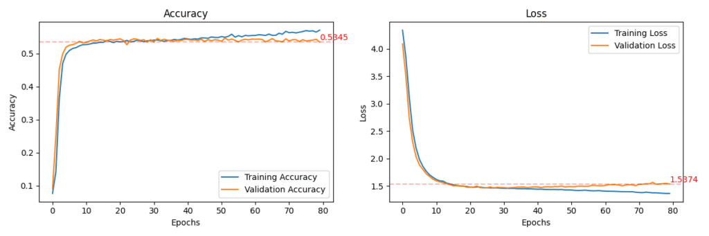
# Step 5: Plot performance
def plot_training_history(history, val_loss, val_acc):
    plt.figure(figsize=(12, 4))

    # Accuracy subplot
    plt.subplot(1, 2, 1)
    plt.plot(history.history['accuracy'], label='Training Accuracy')
    plt.plot(history.history['val_accuracy'], label='Validation Accuracy')
    plt.axhline(y=val_acc, color='r', linestyle='--', alpha=0.3)
    plt.title('Accuracy')
    plt.xlabel('Epochs')
    plt.ylabel('Accuracy')
    plt.legend()
    # Annotate final validation accuracy
    plt.text(len(history.history['accuracy']) - 1, val_acc,
             f'{val_acc:.4f}', color='red', fontsize=10, verticalalignment='bottom')

    # Loss subplot
    plt.subplot(1, 2, 2)
    plt.plot(history.history['loss'], label='Training Loss')
    plt.plot(history.history['val_loss'], label='Validation Loss')
    plt.axhline(y=val_loss, color='r', linestyle='--', alpha=0.3)
    plt.title('Loss')
    plt.xlabel('Epochs')
    plt.ylabel('Loss')
    plt.legend()
    # Annotate final validation loss
    plt.text(len(history.history['loss']) - 1, val_loss,
             f'{val_loss:.4f}', color='red', fontsize=10, verticalalignment='bottom')

    plt.tight_layout()
    plt.savefig('LSTM_Accuracy_Loss.png')
    plt.show()

# Evaluate
val_loss, val_acc = model.evaluate(X_val, y_val, verbose=1)
print(f"\nValidation Accuracy: {val_acc:.4f}")
print(f"Validation Loss: {val_loss:.4f}")

# Plot training performance
plot_training_history(history, val_loss, val_acc)

# Generate sample predictions

def generate_text(seed_text, next_words, model, tokenizer, max_sequence_len):
    for _ in range(next_words):
        token_list = tokenizer.texts_to_sequences([seed_text])[0]
        token_list = pad_sequences([token_list], maxlen=max_sequence_len-1, padding='pre')
        predicted_probs = model.predict(token_list, verbose=0)
        predicted_index = np.argmax(predicted_probs, axis=-1)[0]

        output_word = ""
        for word, index in tokenizer.word_index.items():
            if index == predicted_index:
                output_word = word
                break
        
        # Stop if predicted word is unknown (rare case)
        if output_word == "":
            break

        seed_text += " " + output_word
    return seed_text

print("\nGenerate fashion descriptions:")
seed_input = input("Enter seed text: ")
generated_text = generate_text(seed_input, next_words=10, model=model, tokenizer=tokenizer, max_sequence_len=max_sequence_len)
print(generated_text)

Output:
Generate fashion descriptions:
Enter seed text: A cream coat
A cream coat crafted from cotton for a streetwear look look color silk

There is another variant of RNN. It is called GRU. I will explain in another post named ‘GRU (Gated Recurrent Unit)‘