Hypothesis Testing

Definition :

It is a method of statistical inference used to decide whether the data at hand sufficiently support a particular hypothesis.

Actually we test the assumptions made regarding a population parameter taking support of sample data.

It is generally used when we were to compare:

• a single group with an external standard
• two or more groups with each other

Statistical Test :

There are 2 types of statistical tests:

1. Parametric Statistical Test:-which assumes the shape of the distribution is normal.

   Ex:Z-test.t-test,ANOVA test

2. Non Parametric Statistical test:-It does not assume any shape consideration of samples

   Ex:-Chi square test

Terminology :

1. Null Hypothesis:

• Null hypothesis is a statistical theory that suggests there is no statistical significance exists between the populations.
• It is denoted by H₀ and read as H-naught.
• We have to put claim which is apparently accepted or which equates the system.

2. Alternative Hypothesis:

• An Alternative hypothesis suggests there is a significant difference between the population parameters.
• It is denoted by H_a or H₁
• We have to put the claim which contradicts the Null hypothesis.

          Note:

                   H₀ must always contain equality(=).

                   H_a always contains difference(≠, >, <).

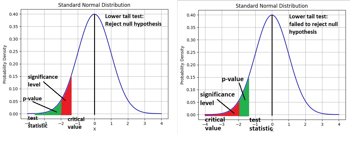
3. Level of significance:

• Denoted by alpha or α.
• It is a fixed probability of wrongly rejecting a True Null Hypothesis.
• For example, if α=5%, that means we are okay to take a 5% risk and conclude there exists a difference when there is no actual difference.

4. Confidence interval :

• Confidence interval describes our uncertainty about where the population mean of a measurement lies, based on a sample.
• It’s calculated using the standard error of the mean. We first choose the confidence level of the interval; usually, we choose the level to be 95%.
• Confidence Level % = 1 − α

5. Point estimate :

• It is a single value estimate of a parameter.
• For instance, a sample mean is a point estimate of a population mean.
• An interval estimate gives you a range of values where the parameter is expected to lie.

6. Critical Value:

• Denoted by C
• It is a value in the distribution beyond which leads to the rejection of the Null Hypothesis.
• It is compared to the test statistic.
• If the value of the test statistic is less extreme than the critical value, then the null hypothesis cannot be rejected.

7. Test Statistic:

• It is denoted by t
• It is dependent on the test that we run.
• It is deciding factor to reject or accept Null Hypothesis.
• Four main test statistics are given below:
  • Z- Score
  • t- Score
  • F-Statistic
  • Chi- Square Statistic

8. p-value :

• It is the probability for the “Null Hypothesis” to be true
• For general cases:
  • If p-value <= 5% ,we reject the null hypothesis.(Alternative hypothesis is accepted).
  • If p-value >= 5% , we fail to reject the null hypothesis.(Null Hypothesis accepted).
• For medical cases:
  • If p-value <= 1% ,we reject the null hypothesis.(Alternative hypothesis is accepted).
  • If p-value >= 1% , we fail to reject the null hypothesis.(Null Hypothesis accepted).

9. Type I Error :

• A Type I error is made if we reject the null hypothesis when it is true (so should have been accepted).
• For example of the person in court, a Type I error would be made if the jury declared the person guilty when they are in fact innocent.

10. Type II Error :

• A Type II error is made if we accept the null hypothesis when it is false i.e. we should have rejected the null hypothesis and accepted the alternative hypothesis.

• This would occur if the jury declared the person innocent when they are in fact guilty.

One sample t-test:

• The one sample t test compares the mean of your sample data to a known value.

Python implementation of one sample t-test:

Claim : Average marriage age of male in India 30 years.

• Hypothesised mean = 30 years

• H₀: The average marriage age of male in india is 30 years

• H_a: The average marriage age of male in india is not 30 years

# importing library

from scipy import stats

# Data collected

mar_age_india = [32,28,29,27,31,32,33,32,35,37,36,25]

# 1 sample ttest

stats.ttest_1samp(mar_age_india,30)

Output:
TtestResult(statistic=1.3428240405418221, pvalue=0.20638105521562627, df=11)

• p value = 0.206 = 20.6%
• As the p-value is greater than 5% , we failed to reject null hypothesis , hence we have to accept it
• The average age of male in india for marriage is 30 years
• Statistic positive , actual average is more than 30

Two sample independent t-test: 

• The two-sample t-test (also known as the independent samples t-test) is a method used to test whether the unknown population means of two groups are equal or not.

Python Implementation of two sample t-test

Claim : Average marriage age of male in India is same as USA

• H₀: Average marriage age of male in India is same as average marriage age in USA

• H_a: Average marriage age of male in India is not same as average marriage age in USA

# importing library

from scipy import stats

# Data Collected

mar_age_india = [32,28,25,29,31,32,33,32,35,32,37]

mar_age_USA = [34,36,39,40,37,35,38,42,38,28,29]

# Two sample independent ttest

stats.ttest_ind(mar_age_india,mar_age_USA)

Output:
Ttest_indResult(statistic=-2.7769208356695327, pvalue=0.011635350464349445)

• P-value = 0.011 = 1.1%

• As the p-value is less than 5% , we reject the null hypothesis.

• We have to accept alternate hypothesis

• So , Average marriage age of male in India is not same as average marriage age in USA

• Also t statistic value is negative , mar_age_india is less than mar_age_USA

Two sample dependent t-test:

• The dependent samples t-test is used to compare the sample means from two related groups.

Python implementation of two sample dependent t-test:

Claim : Effects are same for before drinking redbull & after drinking redbull for response test.

• H₀: Effects are same

• H_a: Effects are not same

# Importing library

from scipy import stats

# Data collected
before_rb = [45,53,66,42,57]
after_rb = [35,42,35,36,32]

# Two sample dependent ttest

stats.ttest_rel(before_rb,after_rb)

Ouput:
TtestResult(statistic=3.4419395040356395, pvalue=0.026247132919799084, df=4)

• p-value = 0.026 = 2.6%
• As P value is less than 5% , we reject the null hypothesis
• We accept the fact that before and after drinking redbull are not same
• As the t statistic is positive , it means response before redbull was high.

ANOVA-One way test:

• Analysis of Variance (ANOVA) is a statistical formula used to compare variances across the means (or average) of different groups.
• In ANOVA we compute a single statistic (an F-statistic) that compares variance between groups with variance within each group.

Formula F = (VAR between)/(VAR within)

• The higher the F-value is, the less probable is the null hypothesis that the samples all come from the same population.

Python implementation for ANOVA:

Claim : All drinks have same effect.

• H₀: All drinks have same effect

• H_a: All drinks have not same effect

# importing library

from scipy import stats

# data collected

lemon = [36,12,46,10,15,20]
coffee = [33,10,38,12,13,19]
redbull = [31,9,39,13,10,15]

# ANOVA One way test

stats.f_oneway(lemon,coffee,redbull)

Ouput:
F_onewayResult(statistic=0.12208729898260585, pvalue=0.8859415816548135)

• P value = 0.885 = 88.5%
• As p value is greater than 5% , we failed to reject the null hypothesis
• We accept null hypothesis that all drinks have same effect

Chi-square test:

• It is a statistical test for categorical data
• It is used to determine whether data are significantly different from what expected.
• It is also called Pearson’s chi-square test
• Chi-square is often written as Χ² and is pronounced “kai-square”
• It is nonparametric tests.
• Formula:

  Χ²=(observed frequency – Expected frequency)2/Expected frequency

• The number of degrees of freedom of the X2 independence test statistics:

          d.f = (rows – 1) x (columns – 1)

• There are two types of Pearson’s chi-square tests:
  • The chi-square goodness of fit test is used to test whether the frequency distribution of a categorical variable is different from expectations.

                  Use for one categorical variable.

                  Example: Ask if ages changed after 10 years for small towns in the US . Where expected based on 10 years before ages & observed based on current ages.

• • The chi-square test of independence is used to test whether two categorical variables are related to each other.

                  Use for two categorical variables.

                  Example: Ask questions if there is the relationship between gender & favorite color. Where there are two categorical variables,a specific type of frequency distribution table is called a contingency table to show the number of observations in each combination of groups.           

How to conclude:

• If chi_square_ value > critical value, the null hypothesis is rejected.
• If chi_square_ value <= critical value, the null hypothesis is failed to reject or accepted.

or

• If p_value > alpha, the null hypothesis is failed to reject or accepted. 
• If p_value <= alpha, the null hypothesis is rejected.

Python implementation of Chi Square test of Independence:

Scenario: Let’s say you are conducting a survey to investigate whether there is a relationship between gender and job satisfaction among employees at a company named XYZ. You collect data from 250 employees, categorizing their responses into three levels of job satisfaction (Satisfied, Neutral, Dissatisfied) and their gender (Male, Female). Your data looks like this:

# import libraries
import numpy as np
import pandas as pd
import seaborn as sns
import scipy.stats as stats
from scipy.stats import chi2


# Create data set

observed_values = np.array([[80, 40, 30],
                                              [30, 30, 40]])


# Define Null & alternative Hypothesis
print("H0 : There is no significant relationship between gender and job satisfaction")
print("Ha : There is a significant relationship between gender and job satisfaction")


# State Alpha

alpha=0.05
print("alpha",alpha)

# Use contingecy function to get p_value,expected values, Chi_square value & degree of freedom

chi_square_value,p_value,dof,expected_values = stats.chi2_contingency(observed_values)

print("chi_square_value :",chi_square_value)
print("p_value :",p_value)
print("dof :",dof)
print("expected_values :",expected_values)


# Getting Critical value

critical_value = chi2.ppf(q=1-alpha,df=dof)  #The ppf() function calculates the percent point function, which gives the value of the test statistic at a certain percentile.
print("critical_value :",critical_value)


# Conclusion from chi_square_statistic

if chi_square_value>critical_value:
     print("Reject the null hypothesis: There is a significant relationship between gender and job satisfaction.")
else:
    print("Fail to reject the null hypothesis: There is no significant relationship between gender and job satisfaction.")

print("---------------------------------------------------------------------------------")

# Conclusion from p-value

if p_value <= alpha:
    print("Reject the null hypothesis: There is a significant relationship between gender and job satisfaction.")
else:
    print("Fail to reject the null hypothesis: There is no significant relationship between gender and job satisfaction.")

Output:
H0 : There is no significant relationship between gender and job satisfaction
Ha : There is a significant relationship between gender and job satisfaction
alpha 0.05
chi_square_value : 16.233766233766232
p_value : 0.0002984574692423908
dof : 2
expected_values : [[66. 42. 42.]
 [44. 28. 28.]]
critical_value : 5.991464547107979
Reject the null hypothesis: There is a significant relationship between gender and job satisfaction.
---------------------------------------------------------------------------------
Reject the null hypothesis: There is a significant relationship between gender and job satisfaction.

Python implementation of Chi Square Goodness of Fit Test:

Scenario: Imagine you are a manager at a clothing store, and you have five different colors of new dress : Pink, Green, Lemon, Raspberry, and Mint. You want to know if the assortment of dress sales matches your expectations based on historical data. You expect the following distribution:

Pink: 40% Green: 20% Lemon: 20% Raspberry: 10% Mint: 10% You collect sales data for a week and want to determine if the actual sales match your expected distribution.

Observed Data:

Pink: 55% Green: 15% Lemon: 15% Raspberry: 5% Mint: 10%

# importing packages
import scipy.stats as stats
import numpy as np

# observed no of hours a student studies in a week vs expected no of hours

observed_data = [40, 20, 20, 10, 10]
expected_data = [55, 15, 15, 5, 10]

# Define Null & alternative Hypothesis
print("H0 : The observed distribution matches the expected distribution")
print("Ha : The observed distribution is different from the expected distribution")

# State Alpha

alpha=0.05
print("alpha",alpha)


# Calculate degree of freedom

dof = len(observed_data)-1
print("degree of freedom :",dof)


# find Chi-Square critical value

critical_value = stats.chi2.ppf(1-alpha, df=dof)
print('critical_value : ', critical_value)


# Chi-Square Goodness of Fit Test

chi_square_statistic, p_value = stats.chisquare(observed_data, expected_data)
print('chi_square_statistic : ',chi_square_statistic)
print('p_value : ',p_value)


# Conclusion from chi_square_statistic

if chi_square_statistic > critical_value:
    print("Reject the null hypothesis: The observed distribution is different from the expected distribution.")
else:
    print("Fail to reject the null hypothesis: The observed distribution matches the expected distribution.")

print("---------------------------------------------------------------------------------")

# Conclusion from p-value

if p_value < alpha:
    print("Reject the null hypothesis: The observed distribution is different from the expected distribution.")
else:
    print("Fail to reject the null hypothesis: The observed distribution matches the expected distribution.")

Ouput:
H0 : The observed distribution matches the expected distribution
Ha : The observed distribution is different from the expected distribution
alpha 0.05
degree of freedom : 4
critical_value :  9.487729036781154
chi_square_statistic :  12.424242424242426
p_value :  0.014460158516237293
Reject the null hypothesis: The observed distribution is different from the expected distribution.
---------------------------------------------------------------------------------
Reject the null hypothesis: The observed distribution is different from the expected distribution