Flow-Based Generative Models
- Flow-based generative models (Normalizing Flows) are a type of deep generative model that learn to model complex probability distributions by transforming a simple distribution (like a normal distribution) into a complex data distribution (e.g., images) using a series of invertible functions.
- Imagine reshaping a blob of clay (simple distribution) into a detailed sculpture (complex distribution) using step-by-step transformations. That’s what flow-based models do, but with data.
How Flow-Based Generative Models Work
- These models rely on normalizing flows, a chain of invertible and differentiable transformations.
- Here’s the basic workflow:
- Start with a simple distribution (e.g., standard normal z ~ N(0,1)).
- Apply a series of transformations (f1, f2, …, fn) to map z to a complex data point x.
- Learn the parameters of the transformations such that the output distribution matches the real data.
Each transformation should be:
- Invertible (you can go from x back to z)
- Differentiable (so gradients can be computed)
Mathematical Intuition
Let’s say:
- is the latent variable (simple Gaussian)
- x = f(z) is the transformed data
- f is a sequence of invertible transformations
To compute the probability of a data point x,
We use the change of variables formula: p(x) = p(z) * ∣ det( ∂z / ∂x )∣
Or rewritten: log p(x) = log p (f−1(x)) + log ∣ det( ∂f−1 / ∂x )∣
This equation is key to flow-based models. We can exactly compute the log-likelihood, which is a major advantage over GANs or VAEs.
Key Terminologies
| Term | Meaning |
|---|---|
| Normalizing Flow | A series of invertible functions to map simple to complex distributions |
| Invertibility | Ability to reverse the transformation |
| Jacobian Determinant | Used to compute how probabilities change after a transformation |
| Latent Variable (z) | A simpler variable that we map from/to the data |
| Base Distribution | Typically Gaussian; starting point of generation |
Types of Flow-Based Models
- Real NVP (Non-Volume Preserving)
- Uses affine coupling layers
- Efficient Jacobian computation
- Glow (Generative Flow)
- Extension of RealNVP with 1×1 convolutions
- Used in image generation
- MAF (Masked Autoregressive Flow)
- Uses autoregressive models to define transformations
- NICE (Nonlinear Independent Components Estimation)
- Early model using additive coupling layers
Applications
| Application | Description |
|---|---|
| Fashion image generation | Generate realistic clothing images |
| Molecular design | Generate molecules with desired properties |
| Audio synthesis | Used in WaveGlow for realistic speech synthesis |
| Anomaly detection | Model normal behavior and detect outliers |
| Style transfer & image editing | Interpretable latent space makes editing intuitive |
Python Implementation for Flow-Based Models
# ---Importing Necessary Libraries---
import torch
import torch.nn as nn
import torch.nn.functional as F
from torchvision.datasets import FashionMNIST
from torchvision.transforms import ToTensor, Normalize, Compose
from torch.utils.data import DataLoader

# --- Conditional Coupling Layer ---
class ConditionalCouplingLayer(nn.Module):
    def __init__(self, in_channels, cond_channels, hidden_dim=128):
        super().__init__()
        self.scale_net = nn.Sequential(
            nn.Conv2d(in_channels // 2 + cond_channels, hidden_dim, kernel_size=3, padding=1),
            nn.ReLU(),
            nn.Conv2d(hidden_dim, in_channels // 2, kernel_size=3, padding=1),
            nn.Tanh()
        )
        self.shift_net = nn.Sequential(
            nn.Conv2d(in_channels // 2 + cond_channels, hidden_dim, kernel_size=3, padding=1),
            nn.ReLU(),
            nn.Conv2d(hidden_dim, in_channels // 2, kernel_size=3, padding=1),
        )

    def forward(self, x, cond, invert=False):
        x1, x2 = x.chunk(2, dim=1)  # split channels into 2 parts
        h = torch.cat([x1, cond], dim=1)  # concat condition on channels

        s = self.scale_net(h)
        t = self.shift_net(h)

        if not invert:
            y2 = x2 * torch.exp(s) + t
        else:
            y2 = (x2 - t) * torch.exp(-s)

        return torch.cat([x1, y2], dim=1)

# --- Simple Conditional Flow Model ---
class ConditionalFlow(nn.Module):
    def __init__(self, in_channels, cond_channels, num_layers=4):
        super().__init__()
        self.layers = nn.ModuleList([
            ConditionalCouplingLayer(in_channels, cond_channels) for _ in range(num_layers)
        ])

    def forward(self, x, cond, invert=False):
        if not invert:
            for layer in self.layers:
                x = layer(x, cond, invert=False)
        else:
            for layer in reversed(self.layers):
                x = layer(x, cond, invert=True)
        return x

# --- Helper: normalize input images and condition ---
transform = Compose([ToTensor(), Normalize((0.5,), (0.5,))])

# --- Load FashionMNIST ---
train_dataset = FashionMNIST(root='./data', train=True, transform=transform, download=True)
train_loader = DataLoader(train_dataset, batch_size=64, shuffle=True)

# --- Function to duplicate channel to get 2 channels ---
def duplicate_channel(x):
    return torch.cat([x, x], dim=1)  # duplicate along channel dim

# --- Instantiate model ---
device = torch.device('cuda' if torch.cuda.is_available() else 'cpu')
in_channels = 2       # doubled channels now
cond_channels = 1     # condition channel remains 1 (original image)
model = ConditionalFlow(in_channels=in_channels, cond_channels=cond_channels).to(device)
optimizer = torch.optim.Adam(model.parameters(), lr=1e-3)

# --- Training Loop ---
epochs = 5
for epoch in range(epochs):
    for x, _ in train_loader:
        cond = x.to(device)            # condition: 1 channel
        target = duplicate_channel(cond)  # target: 2 channels

        z = model(target, cond, invert=False)
        loss = torch.mean(z ** 2)  # encourage latent ~ N(0)

        optimizer.zero_grad()
        loss.backward()
        optimizer.step()

    print(f"Epoch {epoch + 1}/{epochs} Loss: {loss.item():.4f}")

# --- Generate new images conditioned on input ---
model.eval()
with torch.no_grad():
    sample_input, _ = next(iter(train_loader))
    cond_img = sample_input[:1].to(device)               # 1 channel cond image
    z_sample = torch.randn(1, in_channels, 28, 28).to(device)  # latent with 2 channels

    generated_img = model(z_sample, cond_img, invert=True)  # generate image conditioned on cond_img

import matplotlib.pyplot as plt

def show(img_tensor, title=''):
    img = img_tensor.squeeze().cpu().numpy()
    plt.imshow(img, cmap='gray')
    plt.title(title)
    plt.axis('off')
    plt.show()

show(cond_img, title='Condition Image (1 channel)')
show(generated_img[:, 0:1, :, :], title='Generated Image (first channel)')
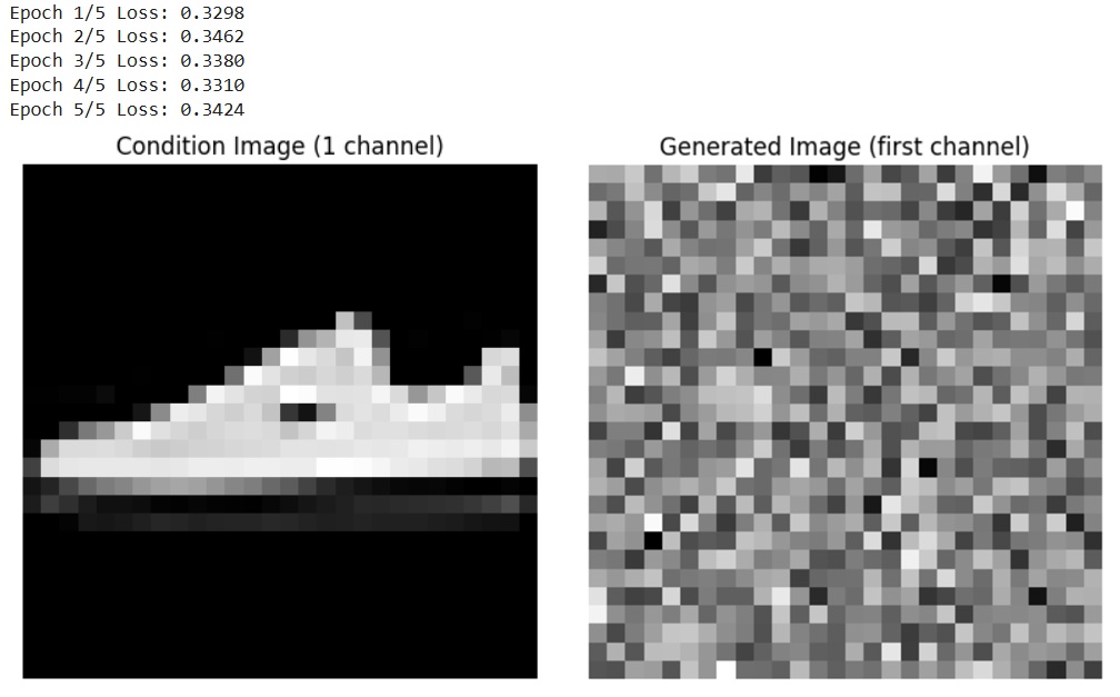
Output Explanation:
From Left Condition Image
- The original FashionMNIST image (1 channel) from the dataset.
- This acts as guidance for generation.
From Right Generated Image (first channel)
- The first channel of the image is generated from a latent sample, conditioned on the input.
- We should expect it to be stylistically or structurally related to the conditioning image.
- For example, if the condition is a sandal, the generated image might also look like a sandal, but with slight variation, as it comes from a random latent.
However, our image may not be visually perfect because:
- The model is simple and only trained for 5 epochs.
- Only 4 coupling layers are used.
- FashionMNIST images are grayscale and low-resolution (28×28), so generation is inherently limited.
References
- Weng, Lilian. “Flow-based Deep Generative Models.“ Lilian Weng’s Blog, October 13, 2018.
- Wang, Dixin, et al. “Flow Matching Models.” arXiv preprint arXiv:2502.13394, 2025. Available at: https://arxiv.org/abs/2502.13394
