Feedforward Neural Networks (FNN)

Feedforward Neural Networks (FNN)

• A Feedforward Neural Network (FNN) is the simplest form of artificial neural network used in supervised learning.
• The data moves in only one direction—forward—from input to output through one or more hidden layers, without any loops or cycles.
• Each neuron in one layer connects to all neurons in the next layer, forming a layered structure.
• These networks are foundational in machine learning and serve as a base for more complex models like CNNs, RNNs, and LSTMs.
• It is also called Vanilla Neural Network, as it is the most basic form of a neural network

Why Use Neural Networks?

Neural networks are powerful because they can:

• Learn non-linear patterns in data that traditional models struggle with.
• Automatically extract features, reducing the need for manual feature engineering.
• Handle large, high-dimensional data like images, text, and time series.
• Generalize well with enough data and proper regularization.

Neural Network Architecture & How It Works

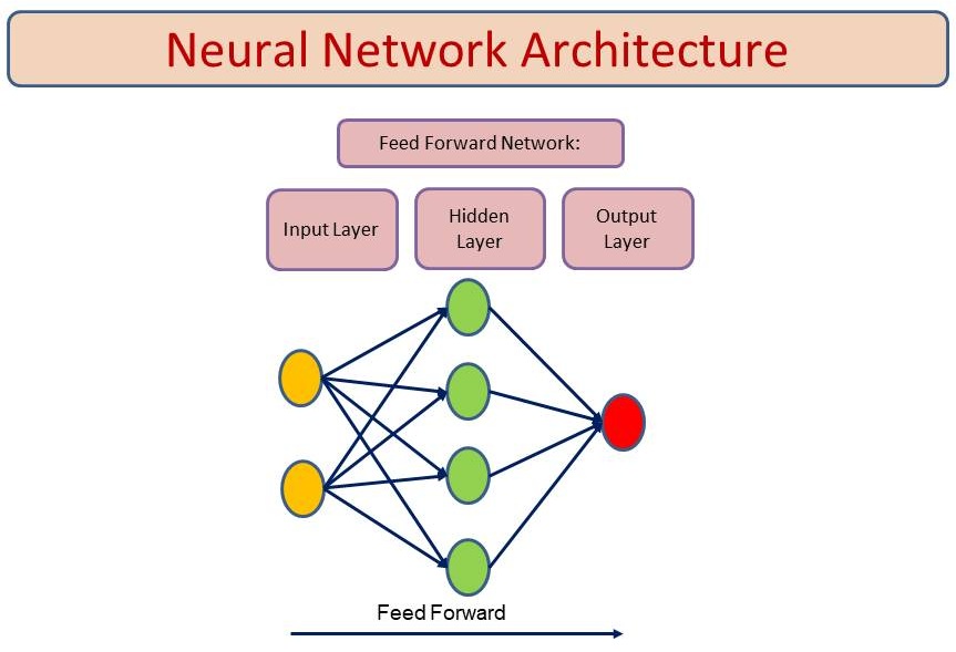
A typical FNN consists of:

• Input Layer
  • Receives raw data
  • A unique weight value is linked to each input in a neural network.
• Hidden Layer
  • Apply transformations using weights, biases, and activation functions.
  • The transformations begin by multiplying inputs with their weights, adding a bias to the result, and then passing the total value or weighted sum through a non-linear activation function.
• Output Layer – Produces the final prediction (e.g., class probabilities in classification).

How It Works:

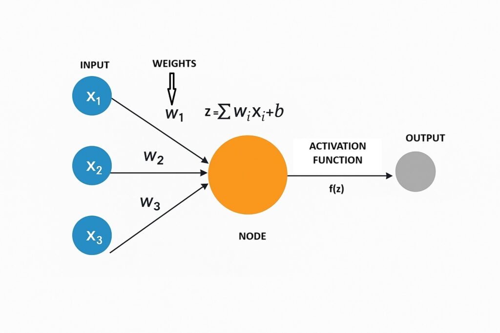
• Forward Propagation:

  • A series of inputs pass through the layer and are multiplied by the weights in this model.
  • In each neuron, weighted input summed together with bias to form weighted sum

    z=w₁​x_1​+w_2​x_2​+…+w_n​x_n​+b,   where w = weights, x = inputs, b = bias.

• • An activation function (e.g., ReLU, Sigmoid) introduces non-linearity: a = f(z). 
  • If the sum exceeds a set threshold (usually zero), the output is 1; otherwise, it’s -1.
    • If sum > threshold (often 0), output = 1.
    • If sum < threshold, output = -1 (binary classification).

• Output Calculation:

  • The final layer produces predictions 
• Calculate loss
  • Use Cross-Entropy for classification, MSE for regression to calculate loss
• Backpropagation:
  • Compute gradients of loss w.r.t. weights.
  • Update weights using Gradient Descent (Minimize the loss function by iteratively adjusting weights)

                    w=w−η⋅∇_wL  where η = learning rate, ∇_wL = gradient of loss.

Activation Functions Used in FNN

Activation functions add non-linearity to the model, allowing it to learn complex functions.

• ReLU (Rectified Linear Unit) – Most common for hidden layers.

                                     f(x)=max⁡ ( 0 , x )

• Sigmoid – Often used for binary classification.         

                                     f(x)=1/ (1+e^−x)

• Softmax – Used in output layer for multi-class classification.

 Python Implementation of a Feedforward Neural Network (FNN)

import tensorflow as tf
from tensorflow.keras import layers, models, datasets
import numpy as np
import matplotlib.pyplot as plt

# Load Fashion-MNIST dataset
(train_images, train_labels), (test_images, test_labels) = datasets.fashion_mnist.load_data()

# Class names for Fashion-MNIST
class_names = ['T-shirt/top', 'Trouser', 'Pullover', 'Dress', 'Coat',
               'Sandal', 'Shirt', 'Sneaker', 'Bag', 'Ankle boot']

# Normalize pixel values to [0, 1]
train_images = train_images / 255.0
test_images = test_images / 255.0

# Build FNN model (MLP with 1 hidden layer)
model = models.Sequential([
    layers.Flatten(input_shape=(28, 28)),  # Input layer (flatten 28x28 image to 784 pixels)
    layers.Dense(128, activation='relu'),   # Hidden layer (128 neurons, ReLU activation)
    layers.Dense(10, activation='softmax')  # Output layer (10 classes, softmax)
])

# Compile the model
model.compile(optimizer='adam',
              loss='sparse_categorical_crossentropy',
              metrics=['accuracy'])

# Train the model
history = model.fit(train_images, train_labels, 
                    epochs=10, 
                    validation_data=(test_images, test_labels))

# Evaluate on test set
test_loss, test_acc = model.evaluate(test_images, test_labels)
print(f"\nTest Accuracy: {test_acc:.4f}")

# Make predictions
predictions = model.predict(test_images)

# Visualize a sample prediction
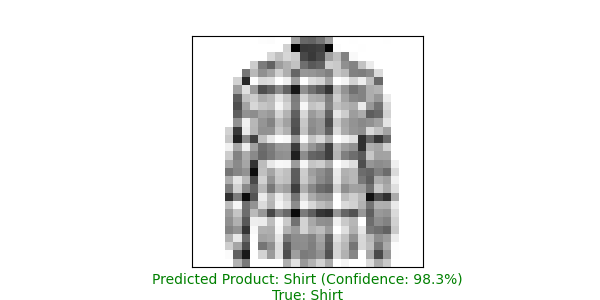
def plot_prediction(i):
    plt.figure(figsize=(6, 3))
    plt.imshow(test_images[i], cmap=plt.cm.binary)
    predicted_label = np.argmax(predictions[i])
    true_label = test_labels[i]
    color = 'green' if predicted_label == true_label else 'red'
    plt.xlabel(f"Predicted Product: {class_names[predicted_label]} (Confidence: {100*np.max(predictions[i]):.1f}%)\nTrue: {class_names[true_label]}", 
               color=color)
    plt.xticks([]); plt.yticks([])
    plt.savefig('prediction.png')
    plt.show()


plot_prediction(7)