
Exploratory Data Analysis (EDA)
- Exploratory Data Analysis (EDA) is an approach to analyzing data sets to summarize their main characteristics, often with visual methods.
- EDA typically involves generating summary statistics for numerical data and visualizing data distributions through histograms, box plots, scatter plots, etc.
- It helps analysts and data scientists understand what the data can tell us beyond the formal modeling or hypothesis-testing tasks.
Univariate Analysis
- Univariate analysis explores each variable in a data set, separately.
- It looks at the range of values, as well as the central tendency of the values.
- It describes the pattern of response to the variable.
- It is quantitative data exploration that we do at the beginning of any analysis.
- The purpose is to make data easier to interpret and to understand how data is distributed within a sample or population being studied.
- Also helps us narrow down exactly what types of bivariate and multivariate analyses we should carry out.
- Univariate Analysis Tools:
- Summary statistics -Determine the value’s center and spread. Like mean, median, standard deviation, etc.
- Frequency table -This shows how frequently various values occur.
- Charts -A visual representation of the distribution of values. Visualizations, such as histograms, distributions, frequency tables, bar charts, pie charts, and boxplots, are also commonly used in univariate analysis.
Bivariate Analysis:
- Bivariate analysis is slightly more analytical than Univariate analysis.
- When the data set contains two variables and researchers aim to undertake comparisons between the two data sets, then Bivariate analysis is the right type of analysis technique.
- This step is performed when the inputs and outputs are known.
- 1st variable will be the Inputs
- 2nd variable will be the output/target variable.
- Bivariate Analysis technique:
Categorical v/s Numerical – sns.barplot(x=data[‘department_name’], y=data[‘length_of_service’])
Numerical v/s Numerical – sns.scatterplot(x=data[‘length_of_service’],y=data[‘age’])
Categorical v/s Categorical – sns.countplot(data[‘STATUS_YEAR’],hue=data[‘STATUS’])
Multivariate Analysis
- It analyzes more than two variables at the same time to understand relationships or patterns.
- Helps find how variables influence each other or group together.
- Common methods like Plot a pair plot with Hue
- sns.heatmap(data.corr(), annot=True)
Python Implementation for EDA:
Importing libraries
import pandas as pd
import numpy as np
import seaborn as sns
import matplotlib.pyplot as plt
%matplotlib inline
Loading Dataset
data = pd.read_csv('/content/drive/MyDrive/Data Science/CDS-07-Machine Learning & Deep Learning/06. Machine Learning Model /07_Support Vector Machines/SVM Class /Test_loan_approved.csv')
See the first five rows
data.head()
Output:
    Loan_ID Gender Married     Education Self_Employed  LoanAmount  Loan_Amount_Term  Credit_History Loan_Status (Approved)
0  LP001002   Male      No      Graduate            No         NaN             360.0             1.0                      Y
1  LP001003   Male     Yes      Graduate            No       128.0             360.0             1.0                      N
2  LP001005   Male     Yes      Graduate           Yes        66.0             360.0             1.0                      Y
3  LP001006   Male     Yes  Not Graduate            No       120.0             360.0             1.0                      Y
4  LP001008   Male      No      Graduate            No       141.0             360.0             1.0                      Y
See the last five rows
data.tail()
Output:
     Loan_ID  Gender Married Education Self_Employed  LoanAmount  Loan_Amount_Term  Credit_History Loan_Status (Approved)
609  LP002978  Female      No  Graduate            No        71.0             360.0             1.0                      Y
610  LP002979    Male     Yes  Graduate            No        40.0             180.0             1.0                      Y
611  LP002983    Male     Yes  Graduate            No       253.0             360.0             1.0                      Y
612  LP002984    Male     Yes  Graduate            No       187.0             360.0             1.0                      Y
613  LP002990  Female      No  Graduate           Yes       133.0             360.0             0.0                      N
See the summary of data
data.info()
<class 'pandas.core.frame.DataFrame'>
RangeIndex: 614 entries, 0 to 613
Data columns (total 9 columns):
 #   Column                  Non-Null Count  Dtype
---  ------                  --------------  -----
 0   Loan_ID                 614 non-null    object
 1   Gender                  601 non-null    object
 2   Married                 611 non-null    object
 3   Education               614 non-null    object
 4   Self_Employed           582 non-null    object
 5   LoanAmount              592 non-null    float64
 6   Loan_Amount_Term        600 non-null    float64
 7   Credit_History          564 non-null    float64
 8   Loan_Status (Approved)  614 non-null    object
dtypes: float64(3), object(6)
memory usage: 43.3+ KB
Insights:
- Data contain object, integer & float data
- There is no null Value
See summary Statistics for numerical variables
data.describe()
Output:
        LoanAmount  Loan_Amount_Term  Credit_History
count  592.000000         600.00000      564.000000
mean   146.412162         342.00000        0.842199
std     85.587325          65.12041        0.364878
min      9.000000          12.00000        0.000000
25%    100.000000         360.00000        1.000000
50%    128.000000         360.00000        1.000000
75%    168.000000         360.00000        1.000000
max    700.000000         480.00000        1.000000
Note: If you find that the standard deviation of a variable is zero, The variable may not be useful for analysis or modeling,
See summary Statistics for Categorical variables
data.describe(include="O")
Output:
        Loan_ID Gender Married Education Self_Employed Loan_Status (Approved)
count        614    601     611       614           582                    614
unique       614      2       2         2             2                      2
top     LP001002   Male     Yes  Graduate            No                      Y
freq           1    489     398       480           500                    422
Insights:
- Male loans are approved the most
- Married people most loan approval
Count the number of unique values in each column
data.nunique()
Loan_ID                   614
Gender                      2
Married                     2
Education                   2
Self_Employed               2
LoanAmount                203
Loan_Amount_Term           10
Credit_History              2
Loan_Status (Approved)      2
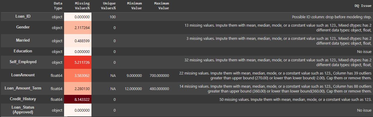
Checking for missing values (null values)
data.isnull().sum()
Loan_ID                    0
Gender                    13
Married                    3
Education                  0
Self_Employed             32
LoanAmount                22
Loan_Amount_Term          14
Credit_History            50
Loan_Status (Approved)     0
Counting the occurrences of each unique value in a Series or a specific column of a DataFrame for a categorical feature
data['Married'].value_counts()
Output:
Yes    398
No     213
Name: Married, dtype: int64
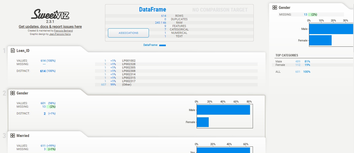
Use a Python package to get an EDA report
- Univariate analysis–sweetviz
# install sweetviz

!pip install sweetviz
Output:
Collecting sweetviz
  Downloading sweetviz-2.3.1-py3-none-any.whl.metadata (24 kB)-----
--------------Successfully installed sweetviz-2.3.1
import sweetviz as sv #  library for univariant analysis

my_report1 = sv.analyze(data)## pass the original dataframe

my_report1.show_html() # Default arguments will generate to "SWEETVIZ_REPORT.html"
Output:
Done! Use 'show' commands to display/save.
 [100%]   00:00 -> (00:00 left)
Report SWEETVIZ_REPORT.html was generated! NOTEBOOK/COLAB USERS: the web browser MAY not pop up, regardless, the report IS saved in your notebook/colab files.
- Bivaraite analysis–Autoviz
# install autoviz

!pip install autoviz
Output:
Collecting autoviz
  Downloading autoviz.........
from autoviz import AutoViz_Class
AV = AutoViz_Class()

bivariate_report = AV.AutoViz('/content/drive/SVM Class /Test_loan_approved.csv',verbose=1)
Output:
Imported v0.1.905. Please call AutoViz in this sequence:
    AV = AutoViz_Class()
    %matplotlib inline
    dfte = AV.AutoViz(filename, sep=',', depVar='', dfte=None, header=0, verbose=1, lowess=False,
               chart_format='svg',max_rows_analyzed=150000,max_cols_analyzed=30, save_plot_dir=None)
Shape of your Data Set loaded: (614, 9)

########## C L A S S I F Y I N G  V A R I A B L E S  ##############
Classifying variables in data set...
    Number of Numeric Columns =  2
    Number of Integer-Categorical Columns =  0
    Number of String-Categorical Columns =  0
    Number of Factor-Categorical Columns =  0
    Number of String-Boolean Columns =  5
    Number of Numeric-Boolean Columns =  1
    Number of Discrete String Columns =  0
    Number of NLP String Columns =  0
    Number of Date Time Columns =  0
    Number of ID Columns =  1
    Number of Columns to Delete =  0
    9 Predictors classified...
        1 variable(s) removed since they were ID or low-information variables
        List of variables removed: ['Loan_ID']
To fix these data quality issues in the dataset, import FixDQ from autoviz...
    All variables classified into correct types.
Number of All Scatter Plots = 3
All Plots done
Time to run AutoViz = 2 seconds

 ###################### AUTO VISUALIZATION Completed ########################
Manual Plotting:
#For Numerical data

import matplotlib.pyplot as plt
import seaborn as sns

plt.figure(figsize=(8,7), facecolor='white')#To set canvas
plotnumber = 1#counter

dataN = data[['LoanAmount',"Loan_Amount_Term","Credit_History"]] # create new dataframe with numerical column

for column in dataN.columns:#accessing the columns
    if plotnumber<=4 :
        ax = plt.subplot(2,2,plotnumber)
        sns.histplot(x=dataN[column],hue=data['Loan_Status (Approved)'])
        plt.xlabel(column,fontsize=10)#assign name to x-axis and set font-20
        plt.ylabel('Loan Status',fontsize=10)
        plt.title('Loan status')
        plotnumber+=1#counter increment
plt.tight_layout()
plt.show()

# For Categorical data

dataC = data[['Gender',"Married","Education","Self_Employed"]] # create new dataframe with numerical column

plt.figure(figsize=(7,8), facecolor='white')#To set canvas
plotnumber = 1#counter

for column in dataC:#accessing the columns
    ax = plt.subplot(3,3,plotnumber)
    sns.countplot(x=dataC[column],hue=data['Loan_Status (Approved)'])
    plt.xlabel(column,fontsize=10)#assign name to x-axis and set font-20
    plt.ylabel('Loan Status',fontsize=10)
    plotnumber+=1#counter increment
plt.tight_layout()

Multivariate Analysis
sns.pairplot(data.drop('Loan_ID',axis=1))

