Decision Tree:
- Decision tree is a supervised machine learning algorithm that can perform both classification and regression task.
- With ensemble techniques, it performs better.
- This algorithm works by dividing the whole dataset into a tree-like structure based on some rules and conditions, and then gives a prediction based on those conditions where:
- Nodes represent features (attributes)
- Root node is the topmost node in a decision tree. It is the starting point of the tree and represents the entire dataset before any splits are made
- Parent node in a decision tree is a node that splits into one or more child nodes based on a decision rule (like a feature condition).
- Child node is a node that originates from the parent node, as a result of a decision or split based on a feature or condition
- Branch in a decision tree represents the outcome of a decision at a node and connects that node to one of its child nodes.
- Leaf nodes are the end points of the tree — they represent the final output or decision after all splits and branches have been followed.
- Nodes represent features (attributes)
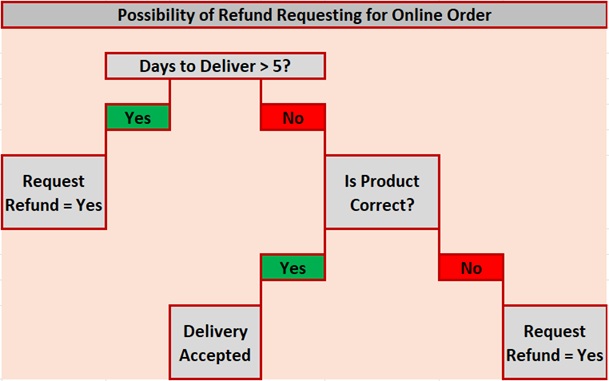
How it works(Explained with Example):
- Selects a root node based on a given condition, e.g. our root node was chosen as Days to deliver is more than 5 days for an online order.
- Then, the root node was split into child nodes based on the given condition.
- The reader’s Left child node in the above figure fulfilled the condition, so no more questions were asked.
- The reader’s right child node didn’t fulfil the condition, so again it was split based on a new condition.
- This process continues till all the conditions are met or if you have predefined the depth of your tree, e.g. the depth of our tree is 3, and it reaches there when all the conditions are exhausted.
Construction of Decision Trees for Regression Task:
In Decision Tree for Regression, the goal is to predict a continuous value (like house price, temperature, etc.) by dividing the feature space into distinct regions and assigning a prediction (typically the mean of the response variable) to each region.
Dividing the Feature Space:
You have a set of input values (X1, X2, …, Xp), which represent your features (like age, income, etc.).
The decision tree algorithm tries to split these input values into non-overlapping regions (R1, R2, …, Rj). Each region contains data points with similar characteristics.
Predicting for Each Region:
After the split, any new data point that falls into a specific region (Rj) will get the mean of the response variable (y) of all training examples in that region.
This means that for each region, the algorithm predicts the average value of the target variable (y) for that region.
Goal – Minimize the Error:
The tree is built in such a way that it minimizes the error between the actual values (y) and the predicted values (mean of y for each region).
The error is measured as the sum of squares of residuals, which represents how far off the predictions are from the actual values.
In the formula:
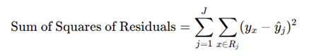
Rj represents a region where the data points are grouped.
yx is the actual value of the response variable for each observation x.
y^j is the predicted value (mean) of the response variable for region .
The goal is to minimize this sum, meaning you want the predicted values to be as close to the actual values as possible.
Imagine we’re trying to predict house prices based on square footage. You split the data into two regions: one for houses with small square footage and another for houses with large square footage.
For small houses, you calculate the average house price in that group.
For large houses, you do the same.
When predicting for a new house:
If the house is small, the tree will predict the average price for small houses.
If the house is large, it will predict the average price for large houses.
Recursive Binary Splitting(Greedy Approach)
- In top-down greedy approach in which nodes are divided into two regions based on the given condition, i.e. not every node will be split, but the ones that satisfy the condition are split into two branches.
- It is called the greedy approach
- In this context, “greedy” means that the algorithm selects the best available option at each step without considering the potential consequences or alternatives that may arise later on.
- In recursive binary splitting, the dataset is split into two subsets at each step based on a chosen feature and a splitting point.
- The goal is to find the best feature and splitting point that minimizes a given criterion, such as reducing the variance or maximizing information gain.
- This continues until a stopping criterion (predefined) is achieved.
- Once all the regions are split, the prediction is made based on the mean of observations in that region.
Construction of Decision Trees for the Classification Task:
- In the case of qualitative data or categorical data, we use classification trees.
- In classification, we split the nodes using classification
- Entropy
- Information Gain
- Gini impurity
Entropy:
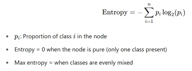
- In the context of decision trees, entropy is a measure of uncertainty or impurity in a node.
- It is calculated by taking the weighted average of the entropies of the child nodes.
- The higher the entropy, the more uncertain or impure the node is.
- The lower the entropy, the more certain or pure the node is.
- Entropy is used to choose the best split for a decision tree.
- The goal is to find a split that reduces the entropy of the node as much as possible.
- This will result in a more pure node, which is easier to classify.
- The formula for calculating entropy is:
Example: Assume,
First child node:
60% of total data
80% in class A → 20% in class B
Second child node:
40% of total data
20% in class A → 80% in class B
Step 1: Compute the entropy of each child
First child:
E1 =−(0.8log2(0.8)+0.2log2(0.2))
=−(0.8⋅(−0.322)+0.2⋅(−2.322))
≈0.722
Second child:
E2 =−(0.2log2(0.2)+0.8log2(0.8))
≈0.722
(Symmetrical distribution, so same entropy.)
Step 2: Weighted average entropy (after split)
Entropy split = 0.6 * 0.722 + 0.4 * 0.722 =0.722
Information Gain:
- In the context of decision trees, information gain is a measure of how much information a feature provides about a class.
- It is calculated by comparing the entropy of the dataset before and after a transformation.
- The feature with the highest information gain is the best feature to split the dataset on.
- The formula for calculating information gain is:
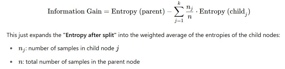
Simplified , InformationGain=Entropy(Before)−Entropy(After)
Where Entropy(Before) is the entropy of the dataset before the transformation, and Entropy(After) is the entropy of the dataset after the transformation.
Example: Assume,
| Weather | Play |
| Sunny | No |
| Sunny | No |
| Overcast | Yes |
| Rain | Yes |
| Rain | Yes |
| Rain | No |
| Overcast | Yes |
| Sunny | Yes |
| Sunny | Yes |
| Rain | Yes |
| Sunny | No |
| Overcast | Yes |
| Overcast | Yes |
| Rain | No |
Total samples = 14
Target: Play (Yes or No)
Step 1: Calculate Entropy of the parent node
Number of “Yes” = 9
Number of “No” = 5
Entropy(Parent) = −((9/14)log2(9/14)+(5/14)log2(5/14)) ≈ 0.940
Step 2: Split by feature (Weather)
Sunny: 5 samples → [2 Yes, 3 No]
Overcast: 4 samples → [4 Yes, 0 No]
Rain: 5 samples → [3 Yes, 2 No]
Entropy(Sunny):
=−((2/5)log2(2/5)+(3/5)log2(3/5)) ≈ 0.971
Entropy(Overcast):
All Yes → Entropy = 0
Entropy(Rain):
=−((3/5)log2(3/5))+(2/5)log2(2/5)) ≈0.971
Step 3: Calculate Weighted Entropy after split
Weighted Entropy = 5/14 * 0.971 + 4/14 * 0+5/14 * 0.971 ≈0.694
Step 4: Calculate Information Gain
Information Gain (Weather) =0.940−0.694 = 0.246
High Information gain = Good feature to split on
Low Information = Less useful, might cause overfitting if used without constraint
Gini Impurity:
- Gini Impurity measures the probability that a randomly chosen item from the set would be incorrectly classified, assuming it was randomly labeled according to the label distribution in the subset.
- The formula for calculating Gini Impurity
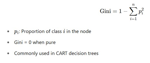
- More misclassification more impurity
Example:
Suppose a node has the following label distribution:
70% class A (p = 0.7)
30% class B (p = 0.3)
Then,
G=1−(0.7²+0.3²)=1−(0.49+0.09)=1−0.58=0.42
So, the Gini Impurity = 0.42
Lower Gini = Better split (purer nodes)
When evaluating possible splits, we choose the feature that reduces Gini impurity the most
Pruning:
- Pruning is a technique that removes parts of the decision tree to reduce complexity and overfitting. In scikit-learn, the ccp_alpha parameter controls cost-complexity pruning, where higher values of ccp_alpha lead to more pruning. The default is ccp_alpha = 0 (no pruning), and typical values like 0.001 or 0.01 are chosen via cross-validation.
Decision Tree Terminologies:
- Root Node: Root Node is from where the decision tree starts.It represents entire dataset,which further gets divided into two or more homogeneous sets
- Leaf Node: Leaf nodes are the final output node and the tree can not be segregated further after getting leaf node.
- Splitting: Splitting is the process of dividing the decision node/root node into sub-nodes according to given conditions.
- Branch/Sub Tree : A tree formed by splitting the tree.
- Pruning: Pruning the process of removing the unwanted branches from tree.
- Parent/Child node: The root node of the tree is called the parent node & other nodes are called as child nodes.
Different Algorithms for Decision Trees
1. ID3 (Iterative Dichotomiser 3)
A foundational algorithm for constructing decision trees for classification.
Uses Information Gain (based on Entropy) as the splitting criterion to select the best attribute at each step.
Only works with categorical features (no support for continuous variables).
Can overfit easily if not pruned properly.
2. C4.5
An improvement over ID3, developed by Ross Quinlan.
Handles both categorical and continuous features.
Uses Gain Ratio instead of plain Information Gain to avoid bias toward features with many categories.
Handles missing values better than ID3.
Performs pruning (specifically, pessimistic pruning), improving generalization.
Still used for classification tasks.
3. CART (Classification and Regression Trees)
One of the most widely used decision tree algorithms.
Supports both classification and regression.
Uses Gini Impurity by default for classification tasks; Mean Squared Error (MSE) for regression.
- In scikit-learn, the DecisionTreeClassifier uses CART under the hood.
- Unlike ID3/C4.5, CART always produces binary trees (splits into two branches at each node).
- You cannot switch between Gini and Entropy within CART itself, but scikit-learn allows you to choose either by setting the criterion parameter (‘gini’ or ‘entropy’).
Advantages of Decision Tree:
- It can be used for both Regression and Classification problems.
- Complex decision tree models are very simple when visualized. It can be understood just by visualising.
- Scaling and normalization are not needed.
Disadvantages of Decision Tree:
- A small change in data can cause instability in the model because of the greedy approach.
- The probability of overfitting is very high for Decision Trees.
- It takes more time to train a decision tree model than other classification algorithms.
Python Implementation for Decision Tree for Classification Task
# Step 1: Import required libraries
from sklearn.tree import DecisionTreeClassifier
from sklearn.model_selection import train_test_split
from sklearn.metrics import classification_report, accuracy_score
from sklearn import datasets
import matplotlib.pyplot as plt
import seaborn as sns
# For Fashion MNIST
from tensorflow.keras.datasets import fashion_mnist
# Step 2: Load the fashion dataset
(X_train, y_train), (X_test, y_test) = fashion_mnist.load_data()
# Step 3: Preprocess data - Flatten the 28x28 images to 784 features
X_train_flat = X_train.reshape(-1, 28 * 28)
X_test_flat = X_test.reshape(-1, 28 * 28)
# Normalize pixel values
X_train_flat = X_train_flat / 255.0
X_test_flat = X_test_flat / 255.0
# Step 4: Train Decision Tree Classifier
model = DecisionTreeClassifier(criterion='gini', max_depth=25, random_state=42)
model.fit(X_train_flat, y_train)
# Step 5: Make predictions
y_pred = model.predict(X_test_flat)
# Step 6: Evaluate performance
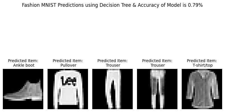
Accuracy = accuracy_score(y_test, y_pred)
# Visualize a few test images with predictions
fashion_labels = ['T-shirt/top', 'Trouser', 'Pullover', 'Dress', 'Coat',
'Sandal', 'Shirt', 'Sneaker', 'Bag', 'Ankle boot']
plt.figure(figsize=(8, 6))
for i in range(5):
plt.subplot(1, 5, i+1)
plt.imshow(X_test[i], cmap='gray')
plt.title(f"Predicted Item:\n {fashion_labels[y_pred[i]]}",fontsize=10)
plt.axis('off')
plt.suptitle(f"Fashion MNIST Predictions using Decision Tree & Accuracy of Model is {Accuracy:.2f}%")
plt.tight_layout()
plt.show()
Python Implementation for Decision Tree for Regression Task
# Step 1: Import necessary libraries
import pandas as pd
import numpy as np
from sklearn.tree import DecisionTreeRegressor
from sklearn.model_selection import train_test_split
from sklearn.metrics import mean_squared_error, r2_score
import matplotlib.pyplot as plt
# Step 2: Loading Dataset
data = pd.read_csv('/content/Clothing_price')
# Step 3: Train/Test Split
X = data.drop('price', axis=1)
y = data['price']
X_train, X_test, y_train, y_test = train_test_split(X, y, test_size=0.2, random_state=42)
# Step 4: Train Decision Tree Regressor
dt_model = DecisionTreeRegressor(max_depth=5, random_state=42)
dt_model.fit(X_train, y_train)
# Step 4: Predictions & Evaluation
y_pred_dt = dt_model.predict(X_test)
plt.figure(figsize=(10, 5))
plt.plot(y_test.values, label='True Price', marker='o')
plt.plot(y_pred_dt, label='DT Predicted', linestyle=':')
r2_dt = r2_score(y_test, y_pred_dt)
mse_dt = mean_squared_error(y_test, y_pred_dt)
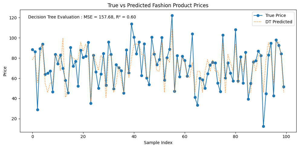
plt.annotate(f"Decision Tree Evaluation : MSE = {mse_dt:.2f}, R² = {r2_dt:.2f}",
xy=(0.03, 0.93),xycoords='axes fraction')
plt.legend()
plt.title("True vs Predicted Fashion Product Prices")
plt.xlabel("Sample Index")
plt.ylabel("Price")
plt.tight_layout()
plt.show()