Association Rule Mining

Association Rule Mining

• Association Rule Mining is a data mining technique used to find interesting relationships (associations) between variables in large datasets.

Goal: Discover rules like:

“If a customer buys Bread and Butter, they are likely to buy Jam.”

This is very common in market basket analysis in retail and e-commerce.

Real-World Example: Fashion Retail

Suppose we’re analyzing shopping patterns in a fashion store:

• Customers who buy denim jackets often also buy white sneakers.

• Customers who buy leggings and sports bras often also buy yoga mats.

This helps with:

• Product placement

• Bundle offers

• Recommendation engines

Basic Terminologies

Let’s define the three key terms: Support, Confidence, and Lift.

1. Support

How often the itemset appears in the dataset.

Support(A) = Transactions containing A / Total transactions​

Example:
Out of 1000 transactions, 100 included “Denim Jacket”.

• Support(Denim Jacket) = 100 / 1000 = 10%

2. Confidence

How often item B is bought when item A is bought.

Confidence(A ⇒ B)=Support(A and B) / Support(A)​

Example:

• 80 customers bought both Denim Jacket and White Sneakers.

• 100 customers bought Denim Jacket.

So,
Confidence(Denim Jacket ⇒ White Sneakers) = 80 / 100 = 80%

3. Lift

How much more likely B is bought when A is bought compared to random chance.

Lift(A ⇒ B)=Confidence(A ⇒ B) / Support(B)​

If Lift > 1: Positive correlation
If Lift = 1: No correlation
If Lift < 1: Negative correlation

Apriori Algorithm

• Apriori is a classical algorithm used to find frequent itemsets and generate association rules from transactional data.

How Apriori Works:

1. Find all frequent itemsets (based on a minimum support threshold).

2. Generate rules from these itemsets (based on minimum confidence and lift).

Steps in Apriori:

1. Scan dataset to count item frequencies.

2. Remove itemsets below support threshold.

3. Combine itemsets to form larger sets.

4. Repeat until no more frequent itemsets.

5. Generate strong rules with high confidence & lift.

Python Implementation for Apriori Algorithm

# Import Necessary Libraries
import pandas as pd
from mlxtend.frequent_patterns import apriori, association_rules

# Sample Data
dataset = [
    ['Denim Jacket', 'White Sneakers'],
    ['Leggings', 'Sports Bra', 'Yoga Mat'],
    ['Denim Jacket', 'White Sneakers', 'Cap'],
    ['Leggings', 'Yoga Mat'],
    ['Denim Jacket', 'Cap'],
]

# Convert to one-hot encoded DataFrame
from mlxtend.preprocessing import TransactionEncoder
te = TransactionEncoder()
te_data = te.fit(dataset).transform(dataset)
df = pd.DataFrame(te_data, columns=te.columns_)

# Step 1: Find Frequent Itemsets
frequent_itemsets = apriori(df, min_support=0.4, use_colnames=True)

# Step 2: Generate Rules
rules = association_rules(frequent_itemsets, metric='confidence', min_threshold=0.6)

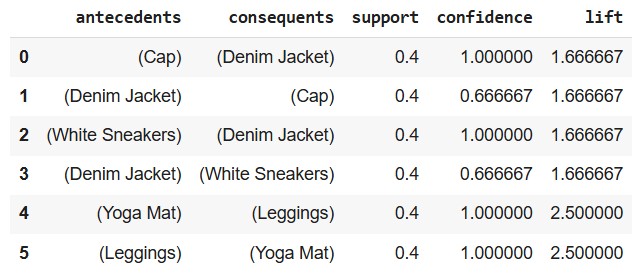
print(rules[['antecedents', 'consequents', 'support', 'confidence', 'lift']])

Insights from the above Table

Row 0

Rule: If Cap, then Denim Jacket

• Support: 0.4 → In 40% of transactions, both Cap and Denim Jacket were bought together.

• Confidence: 1.0 → Every time Cap was bought, Denim Jacket was also bought.

• Lift: 1.67 → Buying a Cap makes the purchase of a Denim Jacket 1.67x more likely than random.

>>> Strong rule with perfect confidence.

Row 1

Rule: If Denim Jacket, then Cap

• Support: 0.4 → Same as above, occurs in 40% of transactions.

• Confidence: 0.67 → 67% of people who bought a Denim Jacket also bought a Cap.

• Lift: 1.67 → Again, this is better than random chance.

>>> Good rule, but not as strong as the reverse.

Row 2

Rule: If White Sneakers, then Denim Jacket

• Support: 0.4 → 40% bought both items.

• Confidence: 1.0 → Everyone who bought White Sneakers also bought a Denim Jacket.

• Lift: 1.67 → Stronger than random chance.

>>> Very strong, could be useful for recommendations.

Row 3

Rule: If Denim Jacket, then White Sneakers

• Confidence: 0.67 → Not all Denim Jacket buyers bought White Sneakers.

• Still decent, and lift says it’s better than chance.

Row 4

Rule: If Yoga Mat, then Leggings

• Support: 0.4 → 40% of people bought both.

• Confidence: 1.0 → 100% who bought Yoga Mat also bought Leggings.

• Lift: 2.5 → Very strong correlation!

>>>  Excellent rule. Yoga Mat buyers are very likely to want Leggings too.

Row 5

Rule: If Leggings, then Yoga Mat

• Same numbers but reversed. Also 100% confidence, 2.5 lift.

>>>Suggests that Yoga-related items are tightly linked.

Now we can:

• Recommend Denim Jacket when someone adds White Sneakers to cart.

• Bundle Cap + Denim Jacket or Leggings + Yoga Mat.

FP-Growth Algorithm 

• FP-Growth is a fast algorithm for mining frequent itemsets without generating candidate itemsets like Apriori does.
• It uses a compact data structure called an FP-tree.

Python Implementation for FP-Growth Algorithm

# Import  Necessary Libraries
from mlxtend.preprocessing import TransactionEncoder
import pandas as pd
from mlxtend.frequent_patterns import fpgrowth
from mlxtend.frequent_patterns import association_rules

# Sample
dataset = [
    ['Denim Jacket', 'White Sneakers'],
    ['Leggings', 'Sports Bra', 'Yoga Mat'],
    ['Denim Jacket', 'White Sneakers', 'Cap'],
    ['Leggings', 'Yoga Mat'],
    ['Denim Jacket', 'Cap']
]

# Convert dataset to one-hot encoded format
te = TransactionEncoder()
te_ary = te.fit(dataset).transform(dataset)
df = pd.DataFrame(te_ary, columns=te.columns_)

# Minimum support can be adjusted (e.g., 0.4 = 40%)
frequent_itemsets = fpgrowth(df, min_support=0.4, use_colnames=True)

# Creating Rules

rules = association_rules(frequent_itemsets, metric="confidence", min_threshold=0.6)

rules[['antecedents', 'consequents', 'support', 'confidence', 'lift']]

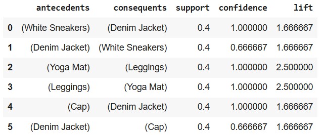
Comparison between Apriori vs FP-Growth