Transfer Learning

Transfer Learning

• Transfer Learning is a machine learning technique where a model developed for one task is reused or adapted as the starting point for another new model, which is designed to perform a related task.
• Instead of training a new model from scratch which can require large amounts of data and computing resources, transfer learning provides knowledge (e.g., learned features, weights, or representations) from a pre-trained model, significantly improving efficiency and performance, especially when labeled data is limited.

Key Concepts:

1. Pre-trained Model: A model previously trained on a large dataset (e.g., ImageNet for images, BERT for text).
2. Fine-tuning: Adjusting the pre-trained model on a new, smaller dataset to specialize it for a different but related task.
3. Feature Extraction: Using the pre-trained model as a fixed feature extractor and training only a new classifier on top.

Analogy:

• Imagine I already know how to ride a bicycle.
• When I decide to learn how to ride a motorcycle, I don’t start completely from scratch because I already understand balance, steering, and how to control speed.
• Instead, I just need to learn the specific controls of the motorcycle.

In the same way:

• A pre-trained model has already learned general “balance and steering” in the form of patterns, features, and representations from a large dataset.
• When applying it to a new but related task, we only need to adjust or fine-tune it to match the new “controls” of your specific problem.

Key Components of Transfer Learning

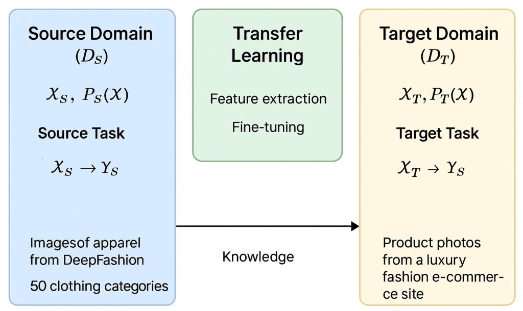
1. Source Domain (D_S)
   • Defined by a feature space X_S and a marginal probability distribution P_S(X).
   • Example: Images of apparel from the DeepFashion dataset, with attributes like sleeves, necklines, colors, etc.
2. Source Task (T_S)
   • Defined by a label space Y_S and an objective function f_S : X_S→Y_S
   • Example: Classifying images into 50 clothing categories (e.g., T-shirts, jeans, coats).
3. Target Domain (D_T)
   • Defined by a feature space X_T and a marginal probability distribution P_T(X), where X_T ≈ X_S but P_T(X) ≠ P_S(X).
   • Example: Product photos from a small luxury fashion e-commerce site (different lighting, models, and style).
4. Target Task (T_T)
   • Defined by a label space Y_T and objective function f_T : X_T→Y_T, where Y_T ≠ Y_S or labelling granularity differs.
   • Example: Predicting seasonal trends (e.g., “Spring Casual”, “Winter Formal”) from product images.
5. Knowledge Transfer Mechanism
   • Feature Extraction:
     Use a pre-trained CNN (e.g., ResNet trained on DeepFashion) to compute feature vectors ϕ(X), then train a simple classifier on ϕ(X_T).
   • Fine-Tuning:
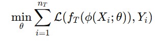
     Minimize

starting from pre-trained weights θ₀ learned on D_S.

Where,

• • • min_θ: We want to find the parameters θ (weights of the neural network) that minimize the total loss on the target dataset.
    • ϕ(X_i ; θ): This is the feature extractor part of the model, parameterized by θ. In transfer learning, ϕ is often a pre-trained network (like ResNet, VGG, BERT) adapted for the new task. Initially, θ comes from the source domain, and we update it slightly during fine-tuning.
    • f_T(⋅): This is the task-specific head (e.g., a fully connected layer for classification) that takes extracted features and outputs predictions for the target task.
    • L(⋅,Y_i) : This is the loss function that measures how far the model’s prediction is from the true label Y_i.

• • Domain Adaptation:
    Adjust feature representations so that P_S(ϕ(X_S)) ≈ P_T(ϕ(X_T)) using techniques like Maximum Mean Discrepancy (MMD) or adversarial alignment.

The goal is to minimize the target risk:   R_T (f_T) = E_(X,Y)∼PT [L(f_T(X),Y)]

using prior knowledge from the source hypothesis f_S to reduce data requirements and improve convergence speed.

Where,

• • f_{T :} The model (or hypothesis) trained or fine-tuned for the target task.

  • (X,Y)∼P_{T :} This means that the input data X and the true labels Y are drawn from the target distribution P_T​.

  • L(f_T(X),Y) : This is the loss function that measures how far the model’s prediction f_T(X)  is from the true label Y.

  • E[⋅] : The expectation is the average loss over all possible samples from the target distribution P_T.

Types of Transfer Learning

1. Inductive Transfer Learning

• Target domain has labeled data (we know the correct outputs for the task).
• The model uses knowledge from the source domain to improve learning on the target domain.

Two types:

• Multi-task Learning:
  • Source and target tasks are trained together.
  • Example: Train one model to recognize faces and emotions at the same time.
• Self-taught Learning:
  • Source domain is unlabeled, but target has labels.
  • Example: Use a large unlabeled dataset of images to learn features, then apply them to classify Fashion-MNIST.

2. Transductive Transfer Learning

• Only source domain has labeled data, target domain has no labels.
• Goal: Apply knowledge from labeled source to unlabeled target.

Two cases:

• Domain Adaptation:
  • Source and target tasks are the same, but domains are different.
  • Example: Train on English reviews (sentiment analysis) → apply to Spanish reviews.
• Covariance Shift:
  • Source and target are from the same domain, but data distribution differs.
  • Example: Train a spam filter on email data from 2010, apply it to emails in 2025 (language patterns shift).

3. Unsupervised Transfer Learning

• Neither source nor target has labeled data.
• Goal: Transfer knowledge to help with unsupervised tasks like clustering, dimensionality reduction, or feature learning.
• Example: Learn useful feature representations from large unlabeled image collections, then apply for grouping images by similarity.

Steps to Implement Transfer Learning

1. Define the Problem & Prepare the Dataset

• Identify the task like classification, regression, object detection, NLP, etc.
• Collect or load the dataset.
• Split into train, validation, and test sets.
• Perform data preprocessing ( data cleaning, resizing, normalization, augmentation, tokenization for NLP, etc.).

2. Choose a Pretrained Model

• Choose a model pretrained on a large dataset that is suitable for our task.
• Popular pretrained models:
  • Vision: ResNet, VGG16, Inception, MobileNetV2.
  • NLP: BERT, RoBERTa, DistilBERT.
• The model we choose should be relevant to our new problem.
• For example, using a model trained on images of animals to classify different species of dogs is a good fit.

3. Feature Extraction

• This is one of the most common approaches in transfer learning. We use the pre-trained model as a fixed feature extractor.
  • Load the model without its top classification layer.
  • Freeze the layers of the pre-trained model. This means their weights will not be updated during training. In this way, weights will remain intact to preserve learned features.
  • This reduces training cost and prevents overfitting when data is small.

4. Add Custom Layers (Fine-tuning Head)

• Add new, trainable layers on top of the frozen base. These layers, often a fully connected layer followed by a dense output layer, will be trained from scratch on your new data to perform the specific classification task.
• Optionally add dropout and batch normalization for generalization.

5. Compile and Train the Model

• Once the model architecture is set up, we’ll compile it with an optimizer (such as Adam or RMSprop) and a loss function suitable for our task (e.g., categorical cross-entropy for multi-class classification).
• Then, train only the new layers we added to your dataset.

6. Fine-Tuning (Optional)

• After training the new layers, we can take it a step further with fine-tuning.
• This process allows the model to adapt its learned features more closely to our specific data.
  • Unfreeze the top layers of the pre-trained base model. It’s best to keep the initial layers frozen, as they contain very general features (like edges and shapes) that are likely relevant to any task.
  • Continue training the entire model (or the unfrozen part) on our data, but with a very low learning rate. This prevents us from destroying the valuable, pre-trained knowledge while allowing the model to make small, incremental adjustments.

Python Implementation for Transfer Learning

# ================================
# STEP 1: Import Libraries
# ================================
import tensorflow as tf
from tensorflow.keras.applications import MobileNetV2
from tensorflow.keras import layers, models
import matplotlib.pyplot as plt

# ================================
# STEP 2: Load Fashion-MNIST Dataset
# ================================
(x_train, y_train), (x_val, y_val) = tf.keras.datasets.fashion_mnist.load_data()

# Expand dims to add channel axis
x_train = tf.expand_dims(x_train, -1)   # shape (60000, 28, 28, 1)
x_val   = tf.expand_dims(x_val, -1)     # shape (10000, 28, 28, 1)

# Convert grayscale → RGB
x_train = tf.image.grayscale_to_rgb(x_train)
x_val   = tf.image.grayscale_to_rgb(x_val)

# Resize to (224,224) for MobileNetV2
x_train = tf.image.resize(x_train, [224,224]) / 255.0
x_val   = tf.image.resize(x_val, [224,224]) / 255.0

# Build tf.data.Dataset
train_ds = tf.data.Dataset.from_tensor_slices((x_train, y_train)).shuffle(10000).batch(32)
val_ds   = tf.data.Dataset.from_tensor_slices((x_val, y_val)).batch(32)

# ================================
# STEP 3: Load Pretrained MobileNetV2
# ================================
base_model = MobileNetV2(
    input_shape=(224, 224, 3),
    include_top=False,
    weights='imagenet'
)

# Freeze base model
base_model.trainable = False

# ================================
# STEP 4: Add Custom Layers
# ================================
model = models.Sequential([
    base_model,
    layers.GlobalAveragePooling2D(),
    layers.Dense(128, activation='relu'),
    layers.Dropout(0.2),
    layers.Dense(10, activation='softmax')   # 10 classes in Fashion-MNIST
])

# ================================
# STEP 5: Compile and Train (Feature Extraction)
# ================================
model.compile(optimizer='adam',
              loss='sparse_categorical_crossentropy',   # labels are integers
              metrics=['accuracy'])

history = model.fit(train_ds, validation_data=val_ds, epochs=5)

# ================================
# STEP 6: Fine-Tuning
# ================================
base_model.trainable = True   # unfreeze

model.compile(optimizer=tf.keras.optimizers.Adam(1e-5),
              loss='sparse_categorical_crossentropy',
              metrics=['accuracy'])

fine_tune_history = model.fit(train_ds, validation_data=val_ds, epochs=5)

# ================================
# STEP 7: Evaluate
# ================================
loss, accuracy = model.evaluate(val_ds)
print(f"Validation accuracy: {accuracy * 100:.2f}%")

# ================================
# STEP 8: Plot Training Curves
# ================================
plt.plot(history.history['accuracy'] + fine_tune_history.history['accuracy'], label='Train Accuracy')
plt.plot(history.history['val_accuracy'] + fine_tune_history.history['val_accuracy'], label='Val Accuracy')
plt.title('Training and Validation Accuracy')
plt.xlabel('Epochs')
plt.ylabel('Accuracy')
plt.legend()
plt.show()

# ================================
# STEP 9: Visualize Sample Images
# ================================
class_names = ['T-shirt/top', 'Trouser', 'Pullover', 'Dress', 'Coat',
               'Sandal', 'Shirt', 'Sneaker', 'Bag', 'Ankle boot']

for images, labels in train_ds.take(1):
    plt.figure(figsize=(10, 10))
    for i in range(9):
        ax = plt.subplot(3, 3, i + 1)
        plt.imshow(images[i].numpy())
        plt.title(class_names[int(labels[i])])
        plt.axis("off")
    plt.show()