
Model Evaluation
- The process of evaluating how well a machine learning model performs on unseen or test data.
- It helps determine whether the model generalizes well beyond the training set.
- In short, it tells how good our model is at making predictions
Importance of Model Evaluation
It helps to
- avoid overfitting or underfitting
- compare different models or algorithms
- ensure the model aligns with real-world performance needs
Types of Evaluation
- Regression problems: Use MAE, MSE, RMSE, or R² score.
- Classification problems: Use accuracy, precision, recall, F1 score, or ROC-AUC.
- Time series or probabilistic models: May use MAPE, log loss, etc.
Model Evaluation Metrics for Regression Model
R² (R-Squared) and Adjusted R²
- R-Squared (R²) is a statistical measure that represents the proportion of the variance in the dependent variable that is predictable from the independent variables.
- It is called R-Squared because it is the square of the correlation coefficient (R) between the observed and predicted values.
- Mathematically, R2 statistic is calculated as :
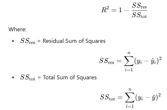
Where,
- yi : Actual value
- yi^: Predicted value from the model
- yˉ: Mean of actual values
- n: Number of observations
- Range: 0 to 1.
- A higher R² indicates a better fit between the model’s predictions and the actual values.
- Interpretation:
- R² = 0.85 means 85% of the variation in the target variable is explained by the model.
- In Python, we can calculate R Square using Sklearn Package(from sklearn.metrics import r2_score)
- Limitation of R²: R² does not account for overfitting. If we keep adding more independent variables, even irrelevant ones, R² may increase artificially, leading to misleading results on the test set.
- Adjusted R² to the Rescue: This is why adjusted R Square is introduced, because it will penalize additional independent variables added to the model and adjust the metric to prevent overfitting issues.
- Mathematical formula, Adjusted R2 = 1 – [(1-R2) * (n-1) / (n-k-1)]
where:
- R2 : The R2 of the model
- n : The number of observations
- k : The number of predictor variables
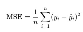
Mean Square Error(MSE)
- While R² is a relative measure of how well the model explains the variance in the dependent variable, Mean Squared Error (MSE) is an absolute measure of the model’s prediction accuracy.
- MSE represents the average of the squared differences between the predicted and actual values:
- In Python, we can use MSE using Sklearn Package from sklearn.metrics import mean_absolute_error
- Interpretation
- MSE gives a concrete value indicating how far off predictions are from actual values.
- While a single MSE value may not be interpretable on its own, it is highly useful for comparing the performance of multiple models.
- A lower MSE indicates a better fit.
RMSE (Root Mean Squared Error)
- RMSE is simply the square root of MSE: RMSE = √MSE
Why use RMSE?
- Interpretable scale:
- Since MSE involves squaring errors, its values can be large.
- Taking the square root brings RMSE back to the same units as the target variable, making it easier to interpret.
- RMSE is more commonly reported than MSE in regression problems due to its direct interpretability.
- In Python, we can use RMSE using sklearn & numpy
mse = mean_squared_error(y_true, y_pred)
rmse = np.sqrt(mse) ,
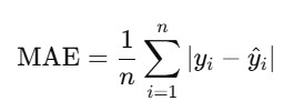
Mean Absolute Error(MAE)
- Mean Absolute Error (MAE) is one of the simplest and most intuitive metrics for evaluating the accuracy of regression models.
- It represents the average of the absolute differences between the predicted values and the actual values:
- Interpretation
- MAE tells you, on average, how much your model’s predictions deviate from the actual values, without considering the direction of the error (positive or negative).
- Unlike MSE, MAE does not square the errors, so it treats all errors equally and is less sensitive to outliers.
- The result is in the same unit as the target variable, making it easy to interpret.
Python Implementation for Regression Evaluation Metrics
import numpy as np
import math
from sklearn.metrics import r2_score, mean_squared_error, mean_absolute_error

# y_test & y_predict from machine learning model  but skipping here as it only evaluation topics explantion

# Evaluation Metrics
print("Evaluation Metrics:")
print("------------------")

# r2 Score
r2 = r2_score(y_test, y_predict)
print('r2:', round(r2, 4))

# Adjusted r2 score
n = 40  # number of samples
k = 3   # number of features (example value)
adjusted_r2 = 1 - (1 - r2) * (n - 1) / (n - k - 1)
print('adjusted_r2:', round(adjusted_r2, 4))

# Mean Square Error (MSE)
MSE = mean_squared_error(y_test, y_predict)
print('MSE:', round(MSE, 4))

# Root Mean Square Error (RMSE)
RMSE = math.sqrt(MSE)
print('RMSE:', round(RMSE, 4))

# Mean Absolute Error (MAE)
MAE = mean_absolute_error(y_test, y_predict)
print('MAE:', round(MAE, 4))
Evaluation Metrics:
------------------
r2: 0.9594
adjusted_r2: 0.9561
MSE: 25.9473
RMSE: 5.0938
MAE: 4.174
Recommendation
- R²/Adjusted R² is useful when explaining the model to others, as it represents the percentage of output variability explained by the model.
- MSE, RMSE, and MAE are better suited for comparing the performance of different regression models.
- RMSE is generally preferred, as it penalizes larger errors more than MAE.
- We can use MSE when the values are not too large.
- We can use MAE when we want to avoid heavily penalizing large errors.
- Adjusted R² is the only metric among these that accounts for overfitting by adjusting for the number of predictors.
Model Evaluation Metrics for Classification Model
- In classification problems, model performance is assessed using a confusion matrix, which shows how accurately the model predicts true positives, true negatives, false positives, and false negatives.
- The different metrics used for this purpose are:
- Accuracy
- Recall/Sensitivity
- Precision
- F1 Score
- Specifity
- AUC( Area Under the Curve)
- ROC(Receiver Operator Characteristic)
- Classification Report
Confusion Matrix
- A confusion matrix is a table used to evaluate the performance of a classification model.
- It compares the model’s predicted labels with the actual labels and helps you understand how well your model is classifying each class.
| Actual Positive (1) | Actual Negative (0) | |
|---|---|---|
| Predicted Positive (1) | TP (True Positive) → Model correctly predicts positive class | FP (False Positive) → Model incorrectly predicts positive (Type I error) |
| Predicted Negative (0) | FN (False Negative) → Model incorrectly predicts negative (Type II error) | TN (True Negative) → Model correctly predicts negative class |
Accuracy
- Accuracy is a metric that measures how often a classification model makes correct predictions.
- The mathematical formula is : Accuracy= (TP+TN) / (TP+TN+FP+FN)
- Use Accuracy when:
- The classes are balanced (i.e., the number of instances in each class is roughly equal).
- We want a general idea of how often the model is right.
- Avoid using accuracy alone when:
- The dataset is imbalanced (e.g., 95% class A, 5% class B).
- In this case, a model predicting only class A would get 95% accuracy but be useless.
- We care more about specific outcomes, like catching fraud (focus on recall) or minimizing false alarms (focus on precision).
- The dataset is imbalanced (e.g., 95% class A, 5% class B).
- Example: Imagine a spam email classifier:
- Out of 100 emails: 90 are not spam, 10 are spam.
- The model predicts all 100 as not spam.
Accuracy = 90/100 = 90%
But it missed all actual spam emails (0% recall for spam). So, accuracy looks good but performance is bad.
Recall or Sensitivity
- Recall (also called Sensitivity or True Positive Rate) measures how well a classification model identifies actual positive cases.
- The mathematical formula is: Recall= TP / (TP+FN)
- Use Recall when:
- Missing a positive case is costly or risky.
- We want to minimize false negatives.
- Use Cases Where Recall is Important:
- Medical diagnosis (e.g., cancer detection): It is better to catch all true cases, even if some are false alarms.
- Fraud detection: It is better to flag all potential fraud, even if a few are innocent.
- Example: Imagine a disease test:
- 10 people actually have the disease.
- The model identifies 8 of them correctly (TP = 8) and misses 2 (FN = 2).
Recall=8 / (8+2) = 0.8 = 80%
- So, the model catches 80% of actual positive cases.
Precision
- Precision measures how many of the predicted positive cases were actually correct.
- Mathematically, Precision=TP / (TP+FP)
- Use Precision when:
- False positives are costly or undesirable.
- We want to minimize incorrect positive predictions.
- Use Cases Where Precision is Important:
- Spam detection – avoid marking real emails as spam.
- Email marketing – ensure only high-quality leads are targeted.
- Legal or security alerts – avoid unnecessary actions on false alarms.
- Example: Imagine a spam filter:
- It predicts 10 emails as spam.
- 7 are actually spam (TP = 7), 3 are not (FP = 3).
Precision=7 / (7+3) = 0.7=70%
- So, 70% of the flagged emails were truly spam.
Trade-off between Recall and Precision
For example,
- There are 10 actual defaulters.
- The model predicted 20 people as defaulters.
- Out of those 20, only 10 were defaulters.
- Metrics:
- Recall = 100% → The model found all defaulters.
- Precision = 50% → Only half of the predicted defaulters were correct.
- False Positives = 10 → 10 people were wrongly flagged as defaulters.
- Interpretation
- The model is very sensitive (high recall) but not specific (low precision).
- In a risk-sensitive context, this is a trade-off:
- Good: We didn’t miss any real defaulters (no false negatives).
- Bad: We wrongly labeled 10 innocent people as defaulters (high false positives).
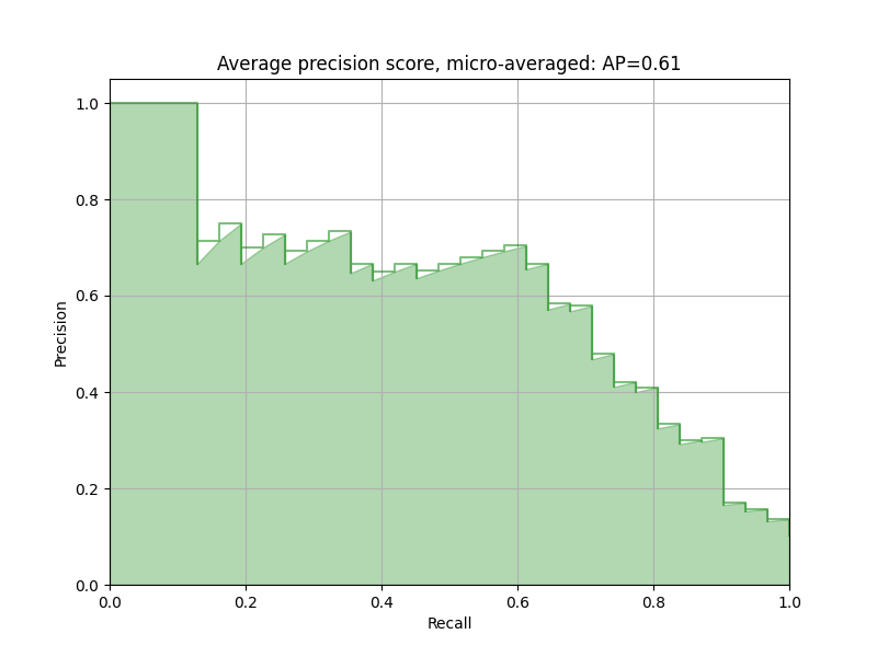
As observed from the graph, when Recall increases, Precision often decreases, and vice versa. This happens because retrieving more actual positives usually comes at the cost of more false positives.
So Which One Should You Focus On?
The answer is: It depends on the business goal.
- If we are predicting cancer, missing a case could cost a life.
→ High Recall is critical: catch all positives, even with some false alarms. - If we are predicting whether someone is innocent, falsely accusing someone is unacceptable.
→ High Precision is essential: only predict positive if we’re sure.
Can We Maximize Both Precision and Recall?
- We can not maximize both precision and recall as there’s usually a trade-off.
- Increasing one often lowers the other.
So, as a solution, a metric that balances both Precision and Recall, F1 Score comes in.
F1 Score
- It is the harmonic mean of Precision and Recall.
- F1 Score is high only when both Precision and Recall are high.
- Best used when you want a balanced view and the class distribution is imbalanced.
- The mathematical formula is: F1 score= (2XPrecisionXRecall) / (Precision+Recall)
Specificity or True Negative Rate
- Specificity (also called the True Negative Rate) measures how well a classification model identifies actual negatives.
- Mathematically, Specificity=TN / (TN+FP)
- It tells us the proportion of actual negative cases that were correctly predicted as negative.
- Use Specificity when:
- It’s important to avoid false positives.
- You want to know how well the model can rule out negative cases.
- Use Cases Where Specificity is Important:
- Medical testing: To confirm that someone does not have a disease.
- Spam filters: To ensure legitimate emails aren’t marked as spam.
- Credit approval systems: To avoid wrongly rejecting trustworthy applicants.
- Example: Suppose you’re building a model to detect fraud:
- Out of 90 non-fraud cases, the model correctly identifies 81 (TN = 81).
- It wrongly flags 9 as fraud (FP = 9).
Specificity=81 (81+9) = 0.9=90%
- So, the model correctly identifies 90% of non-fraud cases.
False Positive rate
- The False Positive Rate (FPR) measures the proportion of actual negative cases that were incorrectly predicted as positive by the model.
- Mathematically: (1- specificity) Or, FP / (TN+FP)
- So, when specificity is high (model correctly identifies negatives), the FPR is low, and vice versa.
- When to Watch FPR:
- Medical screening: A high FPR means many healthy people are incorrectly told they may be sick leading to stress, extra testing, or cost.
- Security systems: High FPR causes false alarms, wasting resources.
- Spam filters: High FPR wrongly flags non-spam emails.
- Example: Out of 100 actual non-defaulters:
- The model wrongly flags 10 as defaulters (FP = 10).
- It correctly identifies 90 as non-defaulters (TN = 90).
FPR=10 / (10+90) = 0.1=10%
- So, 10% of the actual negatives were wrongly flagged.
ROC(Receiver Operator Characteristic)
- In classification tasks, models often predict probabilities rather than definitive class labels. These probabilities range from 0 to 1, where:
- 0 indicates complete certainty of the negative class
- 1 indicates complete certainty of the positive class
- However, real-world data rarely produce perfect 0 or 1 probabilities.
- Instead, predictions fall somewhere in between, like 0.42, 0.76, or 0.88.
- This raises an important question: How do we translate these probabilities into class predictions?
- The answer lies in setting a threshold.
- A threshold is a cutoff point:
- If the predicted probability is above the threshold, the outcome is classified as positive
- If it’s below, it’s classified as negative
For example, with a default threshold of 0.5:
- A prediction of 0.7 becomes a positive class
- A prediction of 0.3 becomes a negative class
But what if your model performs better with a different threshold?
The following diagram shows a typical logistic regression curve.
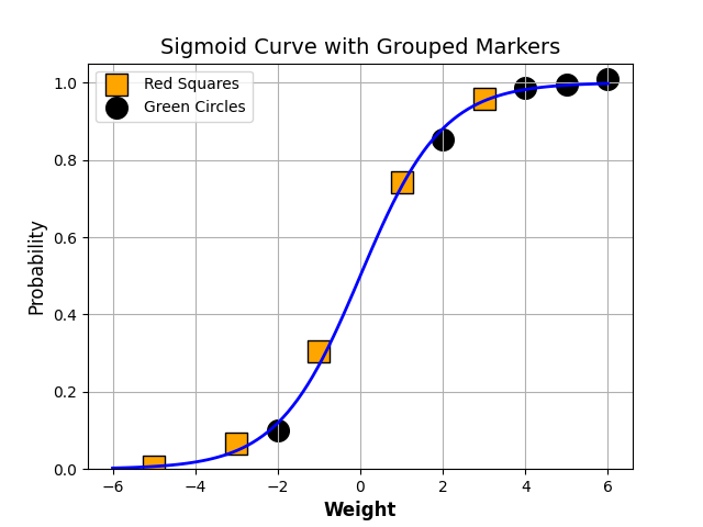
- The horizontal lines represent the various values of thresholds ranging from 0 to 1.
- Let’s suppose our classification problem was to identify the obese people from the given data.
- The black markers represent obese people and the orange markers represent the non-obese people.
- Our confusion matrix will depend on the value of the threshold chosen by us.
- For Example,
- if 0.25 is the threshold then
- TP(actually obese)=3
- TN(Not obese)=2
- FP(Not obese but predicted obese)=2(the two orange squares above the 0.25 line)
- FN(Obese but predicted as not obese )=1(black circle below 0.25line )
- if 0.25 is the threshold then
This illustrates how the choice of threshold directly influences model accuracy, precision, and recall, reinforcing the importance of tools like the ROC curve to guide optimal threshold selection.
A typical ROC curve looks like the following figure.
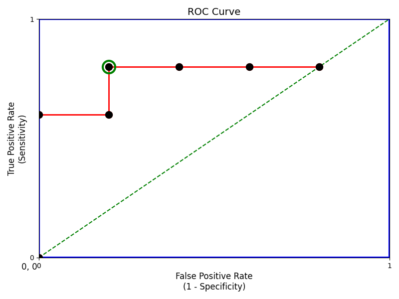
Interpretation of the ROC Curve
- Mathematically, it represents the various confusion matrices for various thresholds. Each black dot is one confusion matrix.
- The green dotted line represents the scenario when the true positive rate equals the false positive rate.
- In the image, as we move from left to right, the false positive rate increases, and the true positive rate initially rises, then drops slightly before leveling off.
- This drop in TPR is not typical but can occur in real-world models due to noisy data or poorly sorted thresholds.
- The green-circled point is still a good operating point. It has a high TPR and lower FPR compared to nearby thresholds.
- But that is not a rule of thumb. Based on the requirement, we need to select the point of a threshold.
- The ROC curve answers our question of which threshold to choose.
AUC(Area Under Curve)
- Suppose that we used different classification algorithms, and different ROCs for the corresponding algorithms have been plotted.
- The question is: which algorithm to choose now? The answer is to calculate the area under each ROC curve.
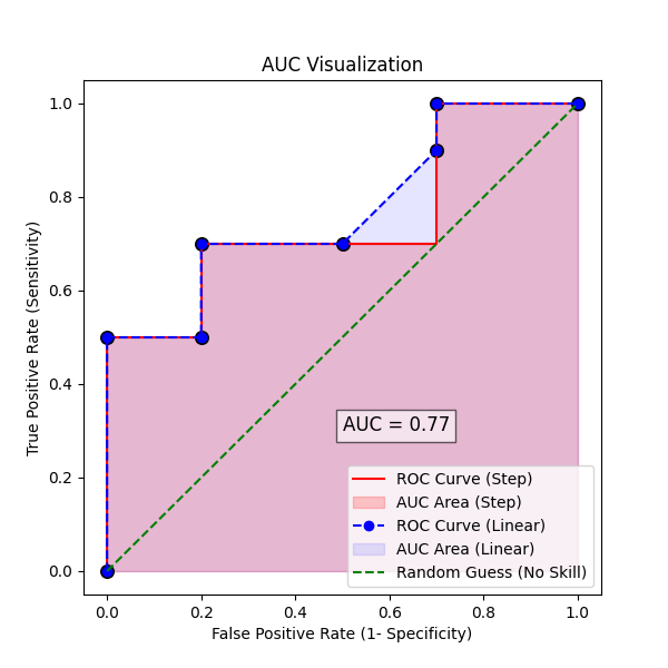
- It helps us to choose the best model amongst the models for which we have plotted the ROC curves
- The best model is the one that encompasses the maximum area under it.
- In the adjacent diagram, the step-wise ROC curve (in red) will encompass the maximum area.
Here’s why:
- The step curve (red) uses the drawstyle=’steps-post’, which means it moves horizontally first (False Positives increase), then vertically (True Positives increase).
- This pattern delays increasing FPR, so the curve stays closer to the top-left corner, which is the ideal zone.
- The linear curve (blue) connects the same points directly, forming triangles instead of rectangles. As a result, it underestimates the true area covered by the ROC.
Classification Report
- A classification report is a summary of key evaluation metrics for a classification model. It includes:
- Precision
- Recall
- F1-score
- Support (The number of actual occurrences of each class in the test data)
- Each of these metrics helps assess your model’s performance per class, offering insight beyond raw accuracy.
- The classification report is especially useful when:
- We have imbalanced classes (e.g., 90% not spam, 10% spam)
- We need to evaluate individual class performance
- We want to compare multiple models
Python Implementation for Classification Evaluation Metrics
from sklearn.datasets import make_classification
from sklearn.model_selection import train_test_split
from sklearn.linear_model import LogisticRegression
from sklearn.metrics import  confusion_matrix, accuracy_score, recall_score, precision_score,classification_report, f1_score, roc_auc_score, roc_curve
import numpy as np

# Generate simple binary classification dataset
X, y = make_classification(n_samples=200, n_features=4, n_informative=2, n_redundant=0, random_state=42)
X_train, X_test, y_train, y_test = train_test_split(X, y, test_size=0.3, random_state=42)

# Train logistic regression model
model = LogisticRegression()
model.fit(X_train, y_train)
y_pred = model.predict(X_test)
y_prob = model.predict_proba(X_test)[:, 1]

# Metrics
cm = confusion_matrix(y_test, y_pred)
accuracy = accuracy_score(y_test, y_pred)
recall = recall_score(y_test, y_pred)
precision = precision_score(y_test, y_pred)
f1 = f1_score(y_test, y_pred)
roc_auc = roc_auc_score(y_test, y_prob)
report = classification_report(y_test, y_pred)

# Extracting TN, FP, FN, TP
tn, fp, fn, tp = cm.ravel()
specificity = tn / (tn + fp)
false_positive_rate = fp / (fp + tn)

# Print all results
print("Confusion Matrix:\n", cm)
print(f"\nAccuracy: {accuracy:.2f}")
print(f"Recall (Sensitivity): {recall:.2f}")
print(f"Precision: {precision:.2f}")
print(f"F1 Score: {f1:.2f}")
print(f"ROC AUC: {roc_auc:.2f}")
print(f"Specificity: {specificity:.2f}")
print(f"False Positive Rate (FPR): {false_positive_rate:.2f}")
print("\nClassification Report:\n", report)
Confusion Matrix:
 [[29  5]
 [ 3 23]]

Accuracy: 0.87
Recall (Sensitivity): 0.88
Precision: 0.82
F1 Score: 0.85
ROC AUC: 0.95
Specificity: 0.85
False Positive Rate (FPR): 0.15

Classification Report:
               precision    recall  f1-score   support

           0       0.91      0.85      0.88        34
           1       0.82      0.88      0.85        26

    accuracy                           0.87        60
   macro avg       0.86      0.87      0.87        60
weighted avg       0.87      0.87      0.87        60
Cross-Validation
- Cross-validation is a resampling technique used to assess the generalizability and performance of a machine learning model on unseen data.
- It helps prevent overfitting by ensuring that the model’s evaluation is not limited to a single train-test split.
- The core idea involves dividing the dataset into multiple subsets, or folds.
- In each iteration, one fold is reserved as the validation set, while the model is trained on the remaining folds.
- This process is repeated until each fold has served as the validation set once.
- The performance metrics from each iteration are then averaged to provide a robust estimate of the model’s effectiveness.
Common Cross-Validation Techniques
K-Fold Cross-Validation
- This is the most widely used method. The data is divided into k equal-sized folds.
- The model is trained on k–1 folds and validated on the remaining fold.
- This process is repeated k times, with each fold used once as the validation set.
- The results from each iteration are then averaged to provide a more robust estimate of the model’s performance than a single train/test split.
- Use k-fold for general-purpose evaluation.
Stratified K-Fold Cross-Validation
- A variation of k-fold is used for classification problems with imbalanced class distributions.
- It ensures each fold maintains the same class proportion as the original dataset, leading to more reliable performance estimates.
- Use stratified k-fold for imbalanced classification tasks.
Leave-One-Out Cross-Validation (LOOCV)
- In LOOCV, each data point is treated as a separate validation set, and the model is trained on the remaining n–1 instances.
- This approach provides an almost unbiased estimate of model performance but is computationally expensive, especially for large datasets.
- Use LOOCV when working with very small datasets.
Repeated K-Fold Cross-Validation
- This method involves repeating the k-fold cross-validation process multiple times with different random splits.
- It helps reduce variance in the performance estimate and is useful when results from a single k-fold run may be unstable.
- Use repeated k-fold for a more stable estimate.
Time Series Cross-Validation (Rolling Forecast Origin)
- Designed for temporal data, where the order of observations is crucial.
- The training set is incrementally expanded, and the model is validated on subsequent time windows.
- This approach respects the temporal structure and avoids data leakage.
- Use time series CV for forecasting and sequential models.
Python Implementation for Cross-Validation Score
1. Classification Example
from sklearn.datasets import load_iris
from sklearn.model_selection import cross_val_score
from sklearn.ensemble import RandomForestClassifier
from sklearn.metrics import make_scorer, f1_score

# Load classification dataset
X, y = load_iris(return_X_y=True)

# Initialize classifier
clf = RandomForestClassifier(random_state=42)

# F1 Score (macro for multi-class)
f1_macro = cross_val_score(clf, X, y, cv=5, scoring='f1_macro')
print("Classification - F1 Macro:", f1_macro)
print("Mean:", f1_macro.mean(), "Std Dev:", f1_macro.std())

# Accuracy
accuracy = cross_val_score(clf, X, y, cv=5, scoring='accuracy')
print("Classification - Accuracy:", accuracy)
print("Mean:", accuracy.mean(), "Std Dev:", accuracy.std())
Classification - F1 Macro: [0.97 0.97 0.93 0.97 1.  ]
Mean: 0.97 Std Dev: 0.02
Classification - Accuracy: [0.97 0.97 0.93 0.97 1.  ]
Mean: 0.97 Std Dev: 0.02
2. Regression Example
from sklearn.datasets import load_diabetes
from sklearn.model_selection import cross_val_score
from sklearn.ensemble import RandomForestRegressor

# Load regression dataset
X, y = load_diabetes(return_X_y=True)
reg = RandomForestRegressor(random_state=42)

# Negative Mean Squared Error (MSE)
mse_scores = cross_val_score(reg, X, y, cv=5, scoring='neg_mean_squared_error')
mse_scores_pos = -mse_scores  # Convert to positive MSE
mse_rounded = np.round(mse_scores_pos, 2)
print("Regression - MSE:", mse_rounded)
print("Mean MSE:", round(mse_scores_pos.mean(), 2), "Std Dev:", round(mse_scores_pos.std(), 2))

# R² Score
r2_scores = cross_val_score(reg, X, y, cv=5, scoring='r2')
r2_rounded = np.round(r2_scores, 2)
print("Regression - R² Score:", r2_rounded)
print("Mean:", round(r2_scores.mean(), 2), "Std Dev:", round(r2_scores.std(), 2))
Regression - MSE: [3006.95 3065.97 3571.39 3405.33 3804.19]
Mean MSE: 3370.77 Std Dev: 301.52
Regression - R² Score: [0.38 0.52 0.43 0.35 0.41]
Mean: 0.42 Std Dev: 0.06
Silhouette Score for Unsupervised Machine learning
So far, we have discussed evaluation metrics for supervised machine learning. Now we will discuss the most common evaluation metrics for unsupervised machine learning
- The Silhouette Score is a widely used metric for evaluating the quality of clustering in unsupervised machine learning.
- It quantifies how well each data point fits within its assigned cluster (cohesion) compared to how well it would fit in the nearest alternative cluster (separation).
The Silhouette Score ranges from -1 to 1:
- A high positive value (close to 1) indicates that the data point is well-matched to its own cluster and poorly matched to neighboring clusters.
- A score near 0 suggests that the data point is on or very close to the decision boundary between two neighboring clusters.
- A negative score (close to -1) indicates that the data point may have been assigned to the wrong cluster.
Python Implementation for Silhouette Score
# Import necessary libraries
from sklearn.cluster import KMeans
from sklearn.metrics import silhouette_score
import numpy as np

# Generate some example data for clustering
data = np.array([[1, 2], [1, 4], [1, 0], [4, 2], [4, 4], [4, 0]])

# Specify the number of clusters you want to test
n_clusters = 2

# Fit a clustering model (e.g., K-Means) to your data
kmeans = KMeans(n_clusters=n_clusters, random_state=0)
cluster_labels = kmeans.fit_predict(data)

# Compute the Silhouette Score
silhouette_avg = silhouette_score(data, cluster_labels)

# Print the Silhouette Score
print(f"Silhouette Score: {silhouette_avg}")
Silhouette Score: 0.17
Model Evaluation Summary
When we use multiple machine learning models, it is easier to see all model performance in a summary table as below
import pandas as pd

df = [['Linear_Regression',0.67,0.45,234,2345,123],['Lasso_Regression',0.67,0.45,234,2345,123],['Ridge_Regression',0.67,0.45,234,2345,123]]

Evaluation_Summary = pd.DataFrame(df,columns=['Model','R2_Score','Adjusted_R2_Score','MSE','RMSE','MAE'])

Evaluation_Summary
	Model	R2_Score	Adjusted_R2_Score	MSE	RMSE	MAE
0	Linear_Regression	0.67	0.45	234	2345	123
1	Lasso_Regression	0.67	0.45	234	2345	123
2	Ridge_Regression	0.67	0.45	234	2345	123
