Diffusion

Diffusion Model

• A diffusion model is a type of deep learning model used to generate new data (such as images) by simulating a two-part process: gradually adding noise to data (forward diffusion) and then learning how to remove that noise (reverse diffusion) to recover or generate meaningful data.
• Think of it like destroying an image step-by-step, then training a model to undo that destruction.
• Inspired by nonequilibrium thermodynamics, where systems move from order to disorder (and ideally back again).
• It has been widely used in powerful tools like DALL·E 3 for text-to-image generation. 

How Diffusion Models Work

1. Forward Diffusion Process (Adding Noise)

• The process begins with a clear image, and random Gaussian noise is added step-by-step over many timesteps.
• As noise accumulates, the image becomes progressively more distorted until it becomes pure noise (like TV static).
• This process is defined by a Markov chain, meaning each step depends only on the previous one.
• A noise scheduler controls how much noise is added at each step.
• After enough steps, the image becomes pure noise & completely unrecognizable.
• Mathematically, the forward process transition probability from x_t−1 to x_t

              q( x_t ​∣ x_t−1 ​) = N(x_t ​; √(1−β_t) *  x_t−1 ​, β_tI)

where,

x₀ = The original clean data sample

x_t = The noised version of the data at step t

x_t−1= The data at the previous step, before adding more noise

N(x;μ,Σ) = A Gaussian distribution with mean μ and covariance Σ

√(1−β_t) *  x_t−1= The mean of the Gaussian scaled version of x_t−1

β_t= The variance schedule, which controls how much noise is added at each step

β_tI= The covariance matrix here, it’s diagonal (i.e., isotropic Gaussian noise)

I= The identity matrix, making the noise equally applied in all directions

2. Reverse Diffusion Process (Removing Noise)

• Now, we train a neural network model that starts with pure noise and learns how to remove the noise in reverse steps to reconstruct the original image.
• This is done using a neural network called a U-Net, which is trained to predict and subtract the noise added in each timestep until the image becomes clear again & turns it into a beautiful image
• The model minimizes the mean squared error(MSE) between the actual and predicted noise.
• Over many steps, the model removes noise in a structured way, revealing the image bit by bit.

• Mathematically, learned reverse transition probability from x_t to x_t−1

         p_θ ​( x_t−1 ​∣ x_t​) = N (x_t−1 ​; μ_θ ​( x_t ​, t ) , Σ_θ​(x_t​,t))

where,

x_t = The noised data at timestep t

x_t−1 = The slightly denoised version (previous step in reverse)

​N(x; μ, Σ) = A Gaussian distribution with mean μ and covariance Σ

μ_θ​ (x_t ​, t) = The predicted mean of the reverse Gaussian learned by the model using x_t and timestep t as inputs.

Σ_θ​(x_t ​, t) = The predicted variance (covariance matrix) also learned by the model. Sometimes it’s fixed or partially learned

θ = The parameters of the neural network trained to model this reverse process.

3. Image Generation (Sampling)

• Start with pure noise
• Use the trained model to gradually remove noise step-by-step and generate a new, realistic image.
• Doesn’t need the same number of steps used in training.
• Fewer steps make the model faster, but with some quality trade-offs.

Conditional or Guided Diffusion (Text-Guided Image Generation)

• So far, the process has been unconditional, meaning no external input guided the image creation.
• Standard diffusion models create random high-quality images.
• However, in real-world use, we often want control, such as generating an image based on a text prompt.
• Guided diffusion allows models to be conditioned (influenced) by specific inputs (like text).
• Text is converted into embeddings or numeric vectors that capture the meaning of the text.
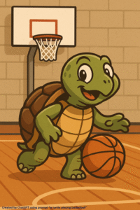
• These embeddings are used to guide the reverse diffusion process, telling the model what kind of image to generate (e.g., “a turtle playing basketball”).
• The model combines a diffusion model with a language model (like CLIP or GPT) to understand the text.

Types of Guided Diffusion

1. Classifier-Guided Diffusion

• Uses a separate classifier to guide the image toward a category.
• Doesn’t need extra training for the diffusion model.
• Limitation: can only guide generation to predefined categories.

2. Classifier-Free Guidance

• No external classifier needed.
• Uses a two-stage model:
  • Stage 1: Use a model like CLIP to turn text into embeddings.
  • Stage 2: Diffusion model uses that embedding to guide the image.
• More flexible → enables zero-shot generation (create new categories it hasn’t seen before).

Latent Diffusion Models

• Standard diffusion is slow and computationally heavy because it works directly on high-resolution images (pixel space).
• Use Latent Diffusion Models (LDMs) like in Stable Diffusion.
• Key idea: Do diffusion in a lower-dimensional latent space instead of pixel space

How Latent Diffusion Models Work

1. Encode the input image into a compressed latent representation (z) using an autoencoder.
2. Apply the diffusion process to this smaller latent version.
3. Use a decoder to convert the denoised latent image back to a full-resolution image.

Applications of Diffusion Models

• Text-to-image generation (e.g., DALL·E)
• Image inpainting (filling missing parts)
• Image-to-image transformation
• Video and audio generation
• Medical imaging, drug discovery, and more

Python Implementation of Diffusion Model

# Import necessary libraries
import tensorflow as tf
from tensorflow.keras import layers, models
import numpy as np
import matplotlib.pyplot as plt

# 1. Load and preprocess Fashion MNIST data
(x_train, _), _ = tf.keras.datasets.fashion_mnist.load_data()
x_train = x_train.astype("float32") / 255.0
x_train = np.reshape(x_train, (-1, 28 * 28))

# 2. Diffusion hyperparameters
timesteps = 200
beta = np.linspace(1e-4, 0.02, timesteps)
alpha = 1. - beta
alpha_hat = np.cumprod(alpha)

# 3. Forward diffusion function
def forward_diffusion_sample(x0, t):
    noise = np.random.randn(*x0.shape)
    sqrt_alpha_hat = np.sqrt(alpha_hat[t])[:, np.newaxis]
    sqrt_one_minus_alpha_hat = np.sqrt(1 - alpha_hat[t])[:, np.newaxis]
    xt = sqrt_alpha_hat * x0 + sqrt_one_minus_alpha_hat * noise
    return xt, noise

# 4. Build simple MLP denoising model
def build_model(input_dim=784):
    inputs = tf.keras.Input(shape=(input_dim + 1,))
    x = layers.Dense(512, activation='relu')(inputs)
    x = layers.Dense(512, activation='relu')(x)
    outputs = layers.Dense(input_dim)(x)
    return models.Model(inputs, outputs)

model = build_model()
model.compile(optimizer='adam', loss='mse')

# 5. Train the model
batch_size = 128
epochs = 5

for epoch in range(epochs):
    for step in range(len(x_train) // batch_size):
        idx = np.random.randint(0, x_train.shape[0], size=batch_size)
        real_images = x_train[idx]
        t = np.random.randint(0, timesteps, size=batch_size)

        xt, noise = forward_diffusion_sample(real_images, t)
        t_normalized = (t / timesteps).reshape(-1, 1)
        xt_input = np.concatenate([xt, t_normalized], axis=1)

        loss = model.train_on_batch(xt_input, noise)

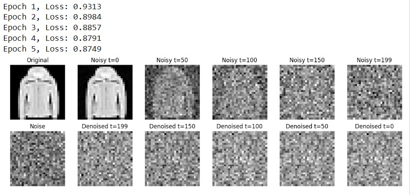
    print(f"Epoch {epoch + 1}, Loss: {loss:.4f}")

# 6. Reverse diffusion with visualization
def sample_and_plot(model, x0, t_steps_to_plot=[0, 50, 100, 150, 199]):
    x = np.random.randn(1, 784).astype(np.float32)
    denoised_steps = []

    for t in reversed(range(timesteps)):
        t_batch = np.full((1, 1), t / timesteps, dtype=np.float32)
        xt_input = np.concatenate([x, t_batch], axis=1)
        noise_pred = model.predict(xt_input, verbose=0)

        beta_t = beta[t]
        alpha_t = alpha[t]
        alpha_hat_t = alpha_hat[t]

        if t > 0:
            noise = np.random.randn(*x.shape)
        else:
            noise = 0

        x = (1 / np.sqrt(alpha_t)) * (
            x - (1 - alpha_t) / np.sqrt(1 - alpha_hat_t) * noise_pred
        ) + np.sqrt(beta_t) * noise

        if t in t_steps_to_plot:
            denoised_steps.append(x.copy())

    return denoised_steps, x

# 7. Visualize forward diffusion and denoising steps
idx = np.random.randint(0, x_train.shape[0])
original = x_train[idx:idx+1]

# Forward noise samples for selected steps
noisy_versions = []
for step in [0, 50, 100, 150, 199]:
    noisy, _ = forward_diffusion_sample(original, np.array([step]))
    noisy_versions.append(noisy)

# Run reverse sampling from noise and collect intermediate denoising steps
denoised_steps, final_img = sample_and_plot(model, original)

# Plot everything
fig, axes = plt.subplots(3, 6, figsize=(12, 6))

# Original + noisy
axes[0, 0].imshow(original.reshape(28, 28), cmap='gray')
axes[0, 0].set_title("Original")
for i, step_img in enumerate(noisy_versions):
    axes[0, i+1].imshow(step_img.reshape(28, 28), cmap='gray')
    axes[0, i+1].set_title(f"Noisy t={ [0,50,100,150,199][i] }")

# Denoising process
axes[1, 0].imshow(np.random.randn(28, 28), cmap='gray')
axes[1, 0].set_title("Noise")
for i, dimg in enumerate(denoised_steps):
    axes[1, i+1].imshow(dimg.reshape(28, 28), cmap='gray')
    axes[1, i+1].set_title(f"Denoised t={ [199,150,100,50,0][i] }")

for row in axes:
    for ax in row:
        ax.axis("off")

plt.tight_layout()
plt.show()

N.B:

Top Row: Forward Diffusion Process

This row shows how the model adds noise to a clean image over a number of time steps:

• Original: The real input image from the Fashion MNIST dataset.
• Noisy t=0: Essentially still looks like the original image.
• Noisy t=50 / 100 / 150 / 199: Gradual increase in noise at t=199, the image is almost completely noise (the final forward diffusion step).

This simulates how the model learns to corrupt an image gradually during training.

Bottom Row: Reverse Denoising (Sampling) Process

This row shows how the model tries to reconstruct an image from pure noise, working backward from t=199 to t=0:

• Noise: Starts from random Gaussian noise (unstructured).
• Denoised t=199 / 150 / … / 0: Intermediate predictions by the model attempting to remove noise step-by-step.
• Denoised t=0: The final output image (should resemble the original).

In our case, the model has not yet been trained enough, so the denoised images still look very noisy. With longer training, the final image  t=0 would gradually resemble the original coat image.

References

1. Ho, J., Jain, A., & Abbeel, P. (2020). Denoising Diffusion Probabilistic Models. Retrieved from https://arxiv.org/abs/2006.11239

2. IBM. (2024). What are Diffusion Models? Retrieved from https://www.ibm.com/think/topics/diffusion-models