What Is an Autoencoder?
Have you ever tried shrinking a big photo so it takes up less space, and then making it big again without losing too much quality? That’s a bit like what an autoencoder does — but with the power of neural networks.
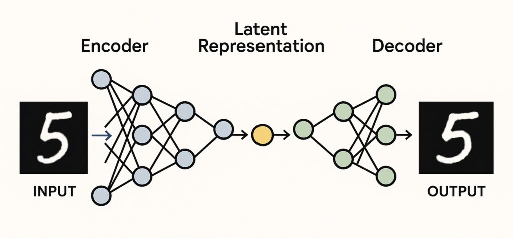
An autoencoder is a special type of machine learning model that learns how to compress data and then rebuild it. It’s made up of two parts:
Encoder: This part squashes the input data (like an image) into a smaller version — a kind of summary or hidden code called a latent representation.
Decoder: This part takes that hidden code and tries to recreate the original input as closely as possible.
Let’s say we give the autoencoder a picture of a handwritten number. First, the encoder turns that picture into a much smaller version that still holds the most important features. Then, the decoder tries to turn that small version back into the original image.
The goal of the autoencoder is to learn how to keep the most useful information while making the smallest possible “summary” of the input. It trains itself by comparing the original input with the output it creates, and trying to reduce the difference (this is called minimizing reconstruction error).
- Image Compression and Denoising
- Autoencoders reduce image size or remove noise by learning key features .
- For example, compressing a photo for faster web loading while preserving clarity.
- Anomaly Detection
- They detect unusual patterns by comparing new data to learned norms.
- For example, identifying fraud in credit card transactions that differ from regular behavior.
- Data Restoration
- Autoencoders can reconstruct missing or corrupted data — for instance, restoring damaged parts of old photographs or filling in missing pixels.
- Synthetic Data Creation
- Autoencoders can be used to generate new synthetic data by learning patterns from the original dataset, especially by using Variational Autoencoders and Generative Adversarial Networks (GAN)
- For example, creating realistic handwritten digits after training on the MNIST dataset. We can even create realistic images of people.
How Autoencoder Works (With Mathematical Intuition):
What Is the Goal?
An autoencoder wants to learn a function that takes an input x and tries to output something as close to x as possible .i.e.,
x^≈x
Here,
- x = original input
- x^ = reconstructed output
The model does this by learning two functions:
- Encoder: z = f(x)
- Decoder: x^ = g(z)
Where:
- f compresses the input into a latent representation z
- g reconstructs the original input from z
Input
We start with some input data, for example, an image of a handwritten digit:
x∈Rn
This is a high-dimensional vector (e.g., 784 pixels for a 28×28 image).
Encoding (Compression)
The encoder maps the input x to a lower-dimensional representation z:
z=f(x)=σ(Wex+be)
- We: weights matrix of the encoder
- be: bias vector
- σ: activation function (e.g., ReLU, sigmoid)
- z∈Rm with m<n: this is the latent representation
This step compresses the input into a more compact format.
Latent Representation
Now we have a bottleneck, a small hidden layer that holds the compressed info:
z=latent code
This bottleneck forces the network to learn only the most important features of the data.
Decoding (Reconstruction)
Now the decoder tries to reconstruct the original input from this compressed code:
x^=g(z)=σ(Wdz+bd)
- Wd: decoder weights
- bd: decoder bias
- x^∈Rn: reconstructed version of input x
This tries to stretch the small code z back into the original input shape.
Reconstruction Loss (Training Objective)
The goal is to make the output x^ as close as possible to the original input x.
So, the network minimizes the reconstruction loss, typically using Mean Squared Error (MSE):
L(x,x^)=∥x−x^∥2
This loss guides how the network updates its weights using gradient descent.
Summary:
Encoder learns how to shrink the data smartly.
Latent space is like a “summary” of your input.
Decoder learns how to expand the summary back.
Loss function helps the network learn what details are important to keep.
Properties of Autoencoders
1. Unsupervised Learning
- Autoencoders do not need labeled data.
- They learn by reconstructing the input, so the target is the input itself:
x→x^
2. Dimensionality Reduction
- The encoder compresses high-dimensional data into a lower-dimensional latent space.
- Similar to PCA, but can model non-linear relationships thanks to neural network layers.
3. Data Reconstruction
- The decoder tries to reconstruct the input from the latent code.
- Performance is evaluated by how well the reconstruction matches the original input.
4. Compression & Feature Extraction
- Autoencoders learn the most important features of the data.
- The latent vector acts as a compact summary or “encoding” of the input.
5. Loss Minimization
- Trained by minimizing reconstruction loss, usually:
- Mean Squared Error (MSE): L=∥x−x^∥2
- Binary Cross-Entropy (for binary images)
6. Architecture Symmetry
- Typically, autoencoders have a symmetric structure:
- Encoder: reduces dimensionality
- Decoder: mirrors the encoder to reconstruct
- Both parts are usually neural networks with similar layer sizes in reverse.
7. Deterministic Mapping
- A basic autoencoder maps an input to a single fixed output (not probabilistic).
- This makes them simpler than models like Variational Autoencoders (VAEs).
8. Noisy Robustness (in Denoising Autoencoders)
- Autoencoders can be trained to remove noise from inputs.
- They learn to reconstruct the original clean data even if the input is corrupted.
9. Limitations
- Can overfit and learn the identity function if:
- The latent space is too large
- There’s no regularization (e.g., sparsity, dropout)
- Not always optimal for generative modeling (better handled by VAEs or GANs)
Variants of Autoencoders
Each variant adds new properties:
- Sparse Autoencoders: enforce sparsity in latent space
- Denoising Autoencoders: trained with noisy input, clean output
- Contractive Autoencoders: penalize sensitivity to input changes
- Variational Autoencoders (VAEs): introduce probabilistic latent space
Key Terms in Autoencoders
Encoder
The part of the autoencoder that compresses the input data into a lower-dimensional form.
Used in representation learning to extract meaningful features from complex data like images or time series.
Decoder
Reconstructs the original input data from the compressed (latent) form.
It learns to “invert” the encoding process.
Code / Bottleneck / Latent Variable
The output of the encoder and input to the decoder; a compact, dense representation of the data.
Often called the latent variable.
In generative models (like Variational Autoencoders), manipulating this code allows generation of new synthetic data.
Latent Space
The space (vector space) where the latent variables live.
It represents the learned feature space, where similar inputs are close together.
Think of it as a hidden layer of understanding, the autoencoder finds abstract patterns here.
Reconstruction
The output generated by the decoder, ideally, a close approximation of the original input.
Loss Function (like MSE or cross-entropy) measures how far off the reconstruction is from the input.
Manifold
The lower-dimensional surface or structure within the higher-dimensional input space where the real data lies.
Autoencoders learn to map inputs to this intrinsic structure of the data.
Manifold learning is at the heart of dimensionality reduction.
Undercomplete Autoencoder
Latent space has fewer dimensions than the input.
Encourages learning meaningful compression instead of just copying the input.
Overcomplete Autoencoder
Latent space has more dimensions than the input.
Needs regularization (e.g., sparsity, denoising) to avoid learning identity function.
Regularization
Techniques (like L1, L2, dropout, or sparsity) used to avoid overfitting or trivial solutions.
Helps the model generalize better by forcing constraints.
Denoising Autoencoder
Trained to reconstruct clean input from a noisy version.
Useful for feature extraction and noise-robust representations.
Sparse Autoencoder
Uses sparsity constraint so that only a few neurons are active at a time in the latent layer.
Good for learning disentangled representations.
Variational Autoencoder (VAE)
A probabilistic model that maps inputs to a distribution over the latent space.
Encourages smoothness and continuity in the latent space, enabling generative modeling.
Reconstruction Loss
A loss function that compares the original input to the reconstruction.
Common: Mean Squared Error (MSE), Binary Cross-Entropy.
KL Divergence (in VAEs)
Measures how much the learned latent distribution deviates from a standard normal distribution.
Part of the VAE loss function to maintain structure in latent space.
Python Implementation of Autoencoder:
# Import Necessary Libraries
import numpy as np
import matplotlib.pyplot as plt
import tensorflow as tf
from tensorflow.keras import layers, models
from PIL import Image
# Creating function Load and preprocess image
def load_and_preprocess_image(img_path, target_size=(128, 128)):
img = Image.open(img_path).convert("RGB")
img = img.resize(target_size)
img_array = np.array(img).astype("float32") / 255.0
return img_array
# Loading my image
img_path = "/content/Original image.jpg"
original_img = load_and_preprocess_image(img_path)
# Prepare training data (just replicate my image many times)
x_train = np.array([original_img for _ in range(500)])
y_train = np.array([original_img for _ in range(500)]) # Target is same image
## Building the Autoencoder Model
input_img = tf.keras.Input(shape=(128, 128 ,3))
# Encoder
x = layers.Conv2D(32, (3, 3), activation='relu', padding='same')(input_img)
x = layers.MaxPooling2D((2, 2), padding='same')(x)
x = layers.Conv2D(16, (3, 3), activation='relu', padding='same')(x)
encoded = layers.MaxPooling2D((2, 2), padding='same')(x)
# Decoder
x = layers.Conv2D(16, (3, 3), activation='relu', padding='same')(encoded)
x = layers.UpSampling2D((2, 2))(x)
x = layers.Conv2D(32, (3, 3), activation='relu', padding='same')(x)
x = layers.UpSampling2D((2, 2))(x)
decoded = layers.Conv2D(3, (3, 3), activation='sigmoid', padding='same')(x)
# Compile the model
autoencoder = models.Model(input_img, decoded)
autoencoder.compile(optimizer='adam', loss='mse')
# Train the autoencoder
autoencoder.fit(x_train, y_train,
epochs=100,
batch_size=32,
shuffle=True)
# Reconstruct the image
reconstructed_img = autoencoder.predict(np.expand_dims(original_img, axis=0))[0]
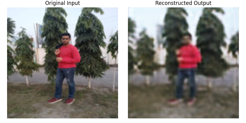
# --- Visualize ---
plt.figure(figsize=(8, 4))
plt.subplot(1, 2, 1)
plt.imshow(original_img)
plt.title("Original Input")
plt.axis('off')
plt.subplot(1, 2, 2)
plt.imshow(reconstructed_img)
plt.title("Reconstructed Output")
plt.axis('off')
plt.tight_layout()
plt.show()
Types of Autoencoders
- Undercomplete Autoencoders
- Regularised Autoencoders
- Sparse Autoencoders
- Denoising Autoencoders
- Contractive Autoencoders
- Convolutional Autoencoder
- Stochastic Autoencoders
- Variational Autoencoders
Undercomplete Autoencoder(Vanilla Autoencoder/Basic Autoencoder)
- An undercomplete autoencoder is a type of autoencoder where the latent (hidden) representation is smaller than the input.
- This forces the model to learn the most important features of the data by compressing it into fewer dimensions.
- It is typically considered the vanilla or basic autoencoder if it is without noise or regularization.
- Use Case:
- Dimensionality reduction: Alternative to PCA for non-linear feature extraction.
- Noise removal: Focuses on capturing the signal, ignoring noise.
- Feature extraction: For downstream tasks like clustering or classification.
- Anomaly detection: Reconstructs normal data well, but fails on unusual patterns.
Pros
- Efficient feature learning: Captures the most relevant data patterns.
- Non-linear dimensionality reduction: Better than PCA for complex data.
- Noise robustness: Learns signal, filters out noise naturally.
Cons
- May lose fine details: Compression can discard subtle features.
- Needs careful architecture tuning: Too small a latent space = underfitting.
- Not ideal for data generation: Can’t generate diverse new samples like Variational Autoencoders (VAEs).
Python Implementation of Undercomplete Autoencoder
# Undercomplete Autoencoder
import tensorflow as tf
from tensorflow.keras.layers import Input, Dense
from tensorflow.keras.models import Model
from tensorflow.keras.datasets import mnist
import numpy as np
# Load and preprocess data
(x_train, _), (x_test, _) = mnist.load_data()
x_train = x_train.astype('float32') / 255.0
x_test = x_test.astype('float32') / 255.0
x_train = x_train.reshape((len(x_train), 784))
x_test = x_test.reshape((len(x_test), 784))
# Define undercomplete autoencoder
input_img = Input(shape=(784,))
encoded = Dense(64, activation='relu')(input_img)
decoded = Dense(784, activation='sigmoid')(encoded)
autoencoder = Model(input_img, decoded)
autoencoder.compile(optimizer='adam', loss='binary_crossentropy')
# Train the model
autoencoder.fit(x_train, x_train,
epochs=20,
batch_size=256,
shuffle=True,
validation_data=(x_test, x_test))
# Encode and decode some digits
reconstructed_imgs = autoencoder.predict(x_test)
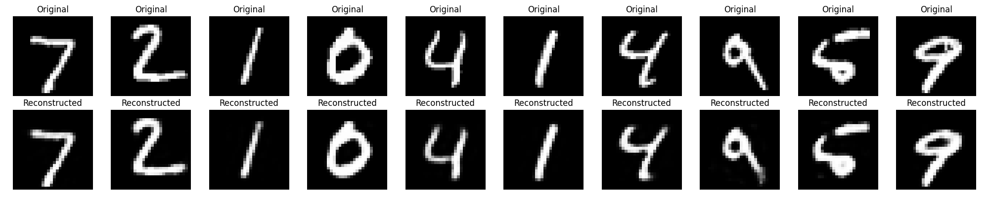
# Visualize original and reconstructed images
n = 10 # Number of digits to display
plt.figure(figsize=(20, 4))
for i in range(n):
# Original images
ax = plt.subplot(2, n, i + 1)
plt.imshow(x_test[i].reshape(28, 28), cmap='gray')
plt.title("Original")
plt.axis('off')
# Reconstructed images
ax = plt.subplot(2, n, i + 1 + n)
plt.imshow(reconstructed_imgs[i].reshape(28, 28), cmap='gray')
plt.title("Reconstructed")
plt.axis('off')
plt.tight_layout()
plt.show()
Regularized Autoencoder?
- A regularized autoencoder is an enhanced version of a standard autoencoder that includes an extra constraint or penalty (regularization term) during training.
- This helps the model learn more meaningful, robust features and avoid overfitting or trivial mappings (e.g., just copying inputs).
There are multiple types, but the most common ones are:
- Sparse Autoencoders
- Encourages the model to activate only a few neurons in the latent (encoded) layer.
- This leads to sparse representations, making the autoencoder focus on the most important features.
- Use Case:
- Feature selection for classification tasks
- Works well for interpretable models, e.g., medical imaging
Pros:
- Helps identify key patterns
- Good for dimensionality reduction
- Useful when explainability is important
- Cons:
- Requires tuning of regularization strength (L1)
- May ignore some useful information if too sparse
- Denoising Autoencoders
- Adds noise to the input and trains the model to reconstruct the original (clean) input.
- This teaches the autoencoder to ignore irrelevant noise.
- Use Case:
- Noise reduction in images or audio
- Robust pretraining for deep learning models
- Pros:
- Handles noisy or corrupted data well
- Improves generalization
- Can be used for data cleaning
- Cons:
- Needs careful choice of noise level
- Might overfit to specific noise patterns if not regularized
Contractive Autoencoders
- Penalizes the model when small changes in the input cause large changes in the encoded output.
- It forces the model to learn smoother and stable representations.
- Use Case:
- Learning important patterns that still work well even if the input data is slightly changed or noisy.
- Applications in signal processing or safety-critical tasks
- Pros:
- Produces robust and stable features
- Helps with smooth decision boundaries
- Cons:
- More computationally expensive due to the added penalty
- Harder to tune than simpler autoencoders
Python Implementation for Sparse, Denoising & Contractive Autoencoder
# Import Necessary Libraries
import numpy as np
import tensorflow as tf
from tensorflow.keras.layers import Input, Dense
from tensorflow.keras.models import Model
from tensorflow.keras.datasets import mnist
from tensorflow.keras import regularizers
import matplotlib.pyplot as plt
# Load and preprocess MNIST
(x_train, _), (x_test, _) = mnist.load_data()
x_train = x_train.astype("float32") / 255.
x_test = x_test.astype("float32") / 255.
x_train = x_train.reshape((-1, 784))
x_test = x_test.reshape((-1, 784))
### === 1. Sparse Autoencoder === ###
input_sparse = Input(shape=(784,))
encoded_sparse = Dense(64, activation='relu',
activity_regularizer=regularizers.l1(1e-5))(input_sparse)
decoded_sparse = Dense(784, activation='sigmoid')(encoded_sparse)
sparse_autoencoder = Model(input_sparse, decoded_sparse)
sparse_autoencoder.compile(optimizer='adam', loss='binary_crossentropy')
### === 2. Denoising Autoencoder === ###
# Add Gaussian noise
noise_factor = 0.3
x_train_noisy = x_train + noise_factor * np.random.normal(loc=0.0, scale=1.0, size=x_train.shape)
x_test_noisy = x_test + noise_factor * np.random.normal(loc=0.0, scale=1.0, size=x_test.shape)
x_train_noisy = np.clip(x_train_noisy, 0., 1.)
x_test_noisy = np.clip(x_test_noisy, 0., 1.)
input_denoise = Input(shape=(784,))
encoded_denoise = Dense(64, activation='relu')(input_denoise)
decoded_denoise = Dense(784, activation='sigmoid')(encoded_denoise)
denoising_autoencoder = Model(input_denoise, decoded_denoise)
denoising_autoencoder.compile(optimizer='adam', loss='binary_crossentropy')
### === 3. Contractive Autoencoder (Custom Loss) === ###
def contractive_loss(y_true, y_pred):
mse = tf.reduce_mean(tf.square(y_true - y_pred))
W = contractive_autoencoder.get_layer('contractive_dense').kernel
h = contractive_autoencoder.get_layer('contractive_dense').output
dh = h * (1 - h) # derivative of sigmoid
contractive_term = tf.reduce_sum(tf.square(W), axis=1)
return mse + 1e-4 * tf.reduce_sum(contractive_term)
input_contract = Input(shape=(784,))
encoded_contract = Dense(64, activation='sigmoid', name='contractive_dense')(input_contract)
decoded_contract = Dense(784, activation='sigmoid')(encoded_contract)
contractive_autoencoder = Model(input_contract, decoded_contract)
contractive_autoencoder.compile(optimizer='adam', loss=contractive_loss)
### === Train All === ###
sparse_autoencoder.fit(x_train, x_train, epochs=10, batch_size=256, shuffle=True,
validation_data=(x_test, x_test))
denoising_autoencoder.fit(x_train_noisy, x_train, epochs=10, batch_size=256, shuffle=True,
validation_data=(x_test_noisy, x_test))
contractive_autoencoder.fit(x_train, x_train, epochs=10, batch_size=256, shuffle=True,
validation_data=(x_test, x_test))
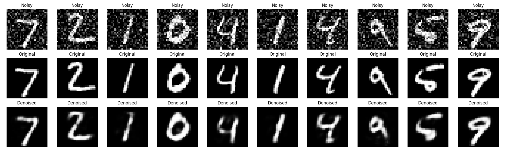
### === Visualize One (e.g., Denoising Result) === ###
decoded_imgs = denoising_autoencoder.predict(x_test_noisy)
n = 10
plt.figure(figsize=(20, 6))
for i in range(n):
# Noisy input
ax = plt.subplot(3, n, i + 1)
plt.imshow(x_test_noisy[i].reshape(28, 28), cmap='gray')
plt.axis('off')
plt.title("Noisy")
# Clean target
ax = plt.subplot(3, n, i + 1 + n)
plt.imshow(x_test[i].reshape(28, 28), cmap='gray')
plt.axis('off')
plt.title("Original")
# Reconstructed
ax = plt.subplot(3, n, i + 1 + 2*n)
plt.imshow(decoded_imgs[i].reshape(28, 28), cmap='gray')
plt.axis('off')
plt.title("Denoised")
plt.tight_layout()
plt.show()
Convolutional Autoencoder
- A Convolutional Autoencoder (CAE) is a type of autoencoder neural network that uses convolutional layers (Conv2D) instead of dense (fully connected) layers to efficiently encode and decode data.
- This makes them ideal for processing images or spatial data.
- It is a powerful deep learning technique for unsupervised learning, often used for tasks like image compression, denoising, and feature extraction.
Use Cases
- Image Denoising
Clean images corrupted with noise by learning patterns and removing unwanted elements. - Image Compression
Reduce image size while retaining key features using learned compact representations. - Anomaly Detection
Detect abnormal patterns by training on normal data and identifying high reconstruction errors. - Dimensionality Reduction
Extract low-dimensional feature vectors from images for tasks like clustering or visualization. - Image Colorization / Inpainting
Reconstruct missing parts or add colors to grayscale images.
- Image Denoising
- Architecture:
Input Image
↓
[Encoder]
– Conv2D -> ReLU
– MaxPooling
↓
Compressed Representation (Latent Space)
↓
[Decoder]
– Conv2DTranspose -> ReLU
– UpSampling
↓
Reconstructed Image
- Pros
- Efficient for image data: Preserves spatial structure better than dense autoencoders.
- Feature Extraction: Can be used to extract deep features for classification or clustering.
- Noise Robustness: Good for denoising applications.
- Unsupervised: Doesn’t need labeled data.
- Cons
- Computationally expensive: Especially with deep networks and large images.
- Data Specific: Needs a lot of training data that is representative of the task.
- Not interpretable: Hard to understand what features are being learned.
- Not ideal for non-image data: Convolutions assume spatial locality.
Python Implementation of Convolutional AutoEncoder
# Importing Necessary Libraries
import numpy as np
import matplotlib.pyplot as plt
from tensorflow.keras.datasets import mnist
from tensorflow.keras.models import Model
from tensorflow.keras.layers import Input, Conv2D, MaxPooling2D, UpSampling2D
from tensorflow.keras.optimizers import Adam
# Load and preprocess MNIST data
(x_train, _), (x_test, _) = mnist.load_data()
x_train = x_train.astype('float32') / 255.
x_test = x_test.astype('float32') / 255.
x_train = np.reshape(x_train, (len(x_train), 28, 28, 1))
x_test = np.reshape(x_test, (len(x_test), 28, 28, 1))
# Encoder
input_img = Input(shape=(28, 28, 1))
x = Conv2D(16, (3, 3), activation='relu', padding='same')(input_img)
x = MaxPooling2D((2, 2), padding='same')(x)
x = Conv2D(8, (3, 3), activation='relu', padding='same')(x)
encoded = MaxPooling2D((2, 2), padding='same')(x)
# Decoder
x = Conv2D(8, (3, 3), activation='relu', padding='same')(encoded)
x = UpSampling2D((2, 2))(x)
x = Conv2D(16, (3, 3), activation='relu', padding='same')(x)
x = UpSampling2D((2, 2))(x)
decoded = Conv2D(1, (3, 3), activation='sigmoid', padding='same')(x)
# Model
autoencoder = Model(input_img, decoded)
autoencoder.compile(optimizer=Adam(), loss='binary_crossentropy')
# Train
autoencoder.fit(x_train, x_train,
epochs=10,
batch_size=128,
shuffle=True,
validation_data=(x_test, x_test))
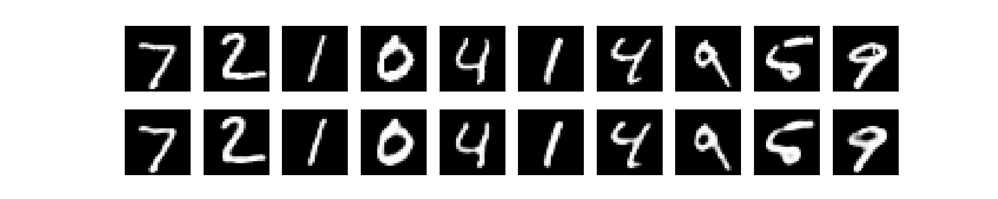
# Visualize
decoded_imgs = autoencoder.predict(x_test)
# Plot original and reconstructed
n = 10
plt.figure(figsize=(20, 4))
for i in range(n):
# original
ax = plt.subplot(2, n, i + 1)
plt.imshow(x_test[i].reshape(28, 28), cmap='gray')
plt.axis('off')
# reconstructed
ax = plt.subplot(2, n, i + 1 + n)
plt.imshow(decoded_imgs[i].reshape(28, 28), cmap='gray')
plt.axis('off')
plt.show()
Stochastic Autoencoder
- A Stochastic Autoencoder is a variant of the autoencoder that introduces randomness (noise or sampling) into the encoding process.
- Unlike traditional deterministic autoencoders, which encode an input into a fixed latent representation, stochastic autoencoders learn a distribution and sample from it to create more robust and generalized representations.
- It encodes an input into a probabilistic distribution, typically a Gaussian (mean and variance).
- Instead of encoding to a fixed point, it samples from this distribution to form the latent representation.
- It learn distributions rather than just compressed representations.
- Generate new data (images, text, etc.) by sampling from the learned latent space.
- The most popular type is the Variational Autoencoder (VAE).
- Use Cases
- Image Generation
Generate new, realistic-looking images after training on a dataset. - Anomaly Detection
Model normal data distributions and detect anomalies based on reconstruction error or low probability. - Denoising
Similar to denoising autoencoders but with better robustness due to latent sampling. - Data Imputation
Fill in missing values by sampling plausible completions from the learned latent space. - Semi-Supervised Learning
Combine labeled and unlabeled data for improved performance using the latent distribution.
- Image Generation
Variational Autoencoder
A VAE consists of three parts:
- Encoder: Maps input to a distribution (mean μ and log-variance logσ²) in a latent space.
- Sampling: Samples from the latent distribution using the reparameterization trick.
- Decoder: Maps the sampled latent vector back to the original input space.
Use Cases of VAE
| Use Case | Description |
|---|---|
| Image Generation | Create new images similar to training images (e.g., fashion items, faces). |
| Anomaly Detection | Detect unusual data points based on reconstruction error. |
| Dimensionality Reduction | Map high-dimensional data to a lower-dimensional latent space. |
| Data Imputation | Fill missing data by sampling from the learned distribution. |
| Semi-supervised Learning | Learn representations even with limited labeled data. |
Pros & Cons of VAE
| Pros | Cons |
|---|---|
| Generates new data samples | May blur outputs (e.g., images) |
| Latent space is smooth and continuous | Complex to tune (e.g., KL weight) |
| Probabilistic: handles uncertainty | Reconstruction may not be sharp |
| Supports sampling and interpolation | KL divergence may dominate training |
Python Implementation of Variational Autoencoder(VAE)
import torch
import torch.nn as nn
import torch.optim as optim
import torch.nn.functional as F
from torchvision import datasets, transforms
from torch.utils.data import DataLoader
import matplotlib.pyplot as plt
# Device config
device = torch.device("cuda" if torch.cuda.is_available() else "cpu")
# Hyperparameters
input_dim = 784 # 28x28
hidden_dim = 400
latent_dim = 20
batch_size = 128
epochs = 10
learning_rate = 0.001
# Load FashionMNIST dataset
transform = transforms.ToTensor()
train_data = datasets.FashionMNIST(root='./data', train=True, download=True, transform=transform)
train_loader = DataLoader(train_data, batch_size=batch_size, shuffle=True)
# Define labels for class names (for recommendation output)
fashion_labels = [
"T-shirt/top", "Trouser", "Pullover", "Dress", "Coat",
"Sandal", "Shirt", "Sneaker", "Bag", "Ankle boot"
]
# VAE Model
class VAE(nn.Module):
def __init__(self, input_dim, hidden_dim, latent_dim):
super(VAE, self).__init__()
self.encoder = nn.Sequential(
nn.Linear(input_dim, hidden_dim),
nn.ReLU(),
nn.Linear(hidden_dim, hidden_dim),
nn.ReLU()
)
self.fc_mu = nn.Linear(hidden_dim, latent_dim)
self.fc_var = nn.Linear(hidden_dim, latent_dim)
self.decoder = nn.Sequential(
nn.Linear(latent_dim, hidden_dim),
nn.ReLU(),
nn.Linear(hidden_dim, hidden_dim),
nn.ReLU(),
nn.Linear(hidden_dim, input_dim),
nn.Sigmoid()
)
def encode(self, x):
h = self.encoder(x)
mu = self.fc_mu(h)
log_var = self.fc_var(h)
return mu, log_var
def reparameterize(self, mu, log_var):
std = torch.exp(0.5 * log_var)
eps = torch.randn_like(std)
return mu + eps * std
def decode(self, z):
return self.decoder(z)
def forward(self, x):
mu, log_var = self.encode(x.view(-1, input_dim))
z = self.reparameterize(mu, log_var)
return self.decode(z), mu, log_var
# Loss
def loss_function(recon_x, x, mu, log_var):
BCE = F.binary_cross_entropy(recon_x, x.view(-1, input_dim), reduction='sum')
KLD = -0.5 * torch.sum(1 + log_var - mu.pow(2) - log_var.exp())
return BCE + KLD
# Initialize model
model = VAE(input_dim, hidden_dim, latent_dim).to(device)
optimizer = optim.Adam(model.parameters(), lr=learning_rate)
# Training loop
def train():
model.train()
train_loss = 0
for batch_idx, (data, _) in enumerate(train_loader):
data = data.to(device)
optimizer.zero_grad()
recon_batch, mu, log_var = model(data)
loss = loss_function(recon_batch, data, mu, log_var)
loss.backward()
train_loss += loss.item()
optimizer.step()
if batch_idx % 100 == 0:
print(f'Train Epoch: {epoch} [{batch_idx * len(data)}/{len(train_loader.dataset)} '
f'({100. * batch_idx / len(train_loader):.0f}%)]\tLoss: {loss.item() / len(data):.6f}')
print(f'====> Epoch: {epoch} Average loss: {train_loss / len(train_loader.dataset):.4f}')
# Training
for epoch in range(1, epochs + 1):
train()
# Define a simple classifier (same input shape as VAE output)
class FashionClassifier(nn.Module):
def __init__(self):
super(FashionClassifier, self).__init__()
self.model = nn.Sequential(
nn.Linear(784, 256),
nn.ReLU(),
nn.Linear(256, 128),
nn.ReLU(),
nn.Linear(128, 10) # 10 FashionMNIST classes
)
def forward(self, x):
return self.model(x)
# Train a classifier on the training set
classifier = FashionClassifier().to(device)
clf_optimizer = optim.Adam(classifier.parameters(), lr=0.001)
criterion = nn.CrossEntropyLoss()
def train_classifier():
classifier.train()
for epoch in range(3): # Quick training for demo
total_loss = 0
for batch_idx, (data, targets) in enumerate(train_loader):
data, targets = data.to(device), targets.to(device)
data = data.view(-1, 784)
clf_optimizer.zero_grad()
outputs = classifier(data)
loss = criterion(outputs, targets)
loss.backward()
clf_optimizer.step()
total_loss += loss.item()
print(f"[Classifier] Epoch {epoch+1} - Loss: {total_loss / len(train_loader):.4f}")
# Train it briefly
train_classifier()
# Generate 1 item and predict its class
with torch.no_grad():
z = torch.randn(1, latent_dim).to(device)
generated = model.decode(z).cpu()
# Predict class from generated image
prediction = classifier(generated.to(device)).argmax(dim=1).item()
label = fashion_labels[prediction]
# Show generated item and label
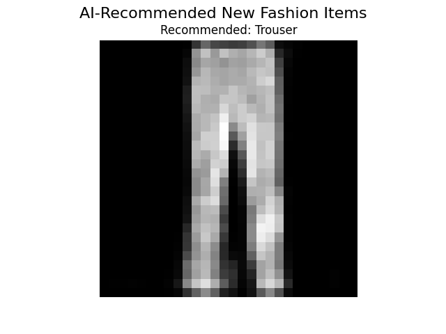
plt.imshow(generated.view(28, 28), cmap='gray')
plt.suptitle("AI-Recommended New Fashion Items", fontsize=16)
plt.title(f"Recommended: {label}")
plt.axis('off')
plt.savefig('generated_item.png')
plt.show()