Gaussian Mixture Model (GMM):
- A Gaussian Mixture Model is a probabilistic model that assumes all the data points are generated from a mixture of several Gaussian distributions, each with unknown parameters.
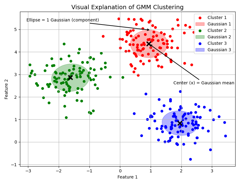
- Think of it as a soft version of clustering, where each data point has a probability of belonging to each cluster, rather than being assigned to just one (as in K-Means).
Imagine we have a bunch of data points that seem to form blobs in different areas of the space. Instead of drawing hard boundaries (like K-Means), you imagine each blob is a bell-shaped curve (a Gaussian). Some points may lie near the center of one blob, others on the edges between blobs.
Why Gaussian?
- Because in the real world (like human heights, measurements, etc.), data often follows a normal (Gaussian) distribution.
- So, a GMM tries to fit several of these “bell curves” to your data.
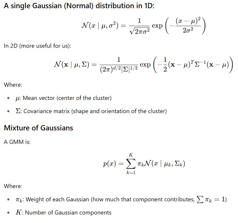
Mathematical Intuition:
How GMM Works:
Step 0: Choose number of components K
Step 1: Assume Data from Gaussians
GMM assumes data points X = {x1,x2,…,xN} are generated from a mixture of K Gaussians.
Each Gaussian has:
mean: μk,
Covariance: Σk,
Weight: πk , where Σ πk=1
Step 2: Expectation-Maximization (EM)
E-Step(Soft Assignment):
For each data point xi, compute the responsibility of each cluster:
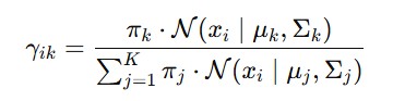
→ It gives the probability that xi came from cluster k
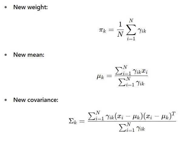
M-Step(Update Parameters):
Update the parameters based on responsibilities:
Step 3: Repeat E and M until convergence (parameters stop changing)
Step 4: Final Cluster Assignment :
Assign each point to the cluster with highest probability
| Term | Meaning |
|---|---|
| μK | Mean of cluster k |
| ΣK | Covariance of cluster k |
| πK | Weight (prior) of cluster k |
| E-step | Compute cluster probabilities (soft assignment) |
| M-step | Update parameters to better fit the data |
| GMM | Probabilistic soft clustering using Gaussian distributions |
Python Implementation for Gaussian Mixture Model:
# Import Necessary Libraries
import pandas as pd
import numpy as np
import matplotlib.pyplot as plt
from matplotlib.patches import Ellipse
from sklearn.mixture import GaussianMixture
from sklearn.preprocessing import StandardScaler
# Step 1: Load your retail dataset
df = pd.read_csv('/content/Mall_Customers.csv')
# Step 2: Select useful features for segmentation
# Example: 'Annual Income' vs. 'Spending Score'
X = df[['Annual Income (k$)', 'Spending Score (1-100)']].values
# Step 3: Standardize the features
scaler = StandardScaler()
X_scaled = scaler.fit_transform(X)
# Step 4: Fit GMM Model
gmm = GaussianMixture(n_components=4, covariance_type='full', random_state=42)
gmm.fit(X_scaled)
# Step 5: Predict cluster labels
labels = gmm.predict(X_scaled)
means = gmm.means_
covs = gmm.covariances_
# Step 6: Function to draw Gaussian ellipse
def draw_ellipse(position, covariance, ax, color):
if covariance.shape == (2, 2):
U, s, Vt = np.linalg.svd(covariance)
angle = np.degrees(np.arctan2(U[1, 0], U[0, 0]))
width, height = 2 * np.sqrt(s)
else:
angle = 0
width, height = 2 * np.sqrt(covariance)
ell = Ellipse(xy=position, width=width, height=height, angle=angle,
color=color, alpha=0.3)
ax.add_patch(ell)
# Step 7: Visualize the results
fig, ax = plt.subplots(figsize=(8, 6))
colors = ['red', 'blue', 'green', 'orange']
for i in range(gmm.n_components):
cluster_data = X_scaled[labels == i]
ax.scatter(cluster_data[:, 0], cluster_data[:, 1], s=30, color=colors[i], label=f'Segment {i+1}')
draw_ellipse(means[i], covs[i], ax, colors[i])
ax.plot(means[i][0], means[i][1], 'kx', markersize=10, mew=3)
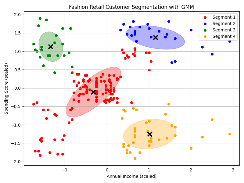
ax.set_title("Fashion Retail Customer Segmentation with GMM")
ax.set_xlabel("Annual Income (scaled)")
ax.set_ylabel("Spending Score (scaled)")
ax.legend()
plt.grid(True)
plt.tight_layout()
plt.savefig('fashion_retail_customer_segmentation.png')
plt.show()