Diving into deep learning for time series can unlock powerful capabilities, especially when traditional models (like ARIMA or XGBoost) fall short due to complexity or scale.
When to Choose Deep Learning:
Complex, non-linear patterns that classical models can’t capture.
Multivariate time series with multiple input variables (features).
Need for long-term memory (e.g., patterns across weeks or months).
Large volumes of data that traditional models can’t handle well.
Real-time or near real-time forecasting at scale.
Example: Predicting sales influenced by promotions, weather, and calendar, all interacting over time.
Common Deep Learning Models for Time Series:
LSTM (Long Short-Term Memory)
Handles long-term dependencies in sequential data.
Good for univariate and multivariate forecasting.
Avoids vanishing gradients better than vanilla RNNs.
Use when: You’re forecasting a value like sales or energy demand and want the model to “remember” what happened several days/weeks ago.
GRU (Gated Recurrent Unit)
Similar to LSTM but with fewer parameters (faster to train).
Slightly less expressive but often performs comparably.
Use when: You want a lighter, faster alternative to LSTM for similar tasks.
CNN for Time Series
Uses convolution to detect local temporal patterns.
Surprisingly effective even without recurrence.
Great for multivariate inputs and short-term patterns.
Use when: You’re dealing with high-frequency data and want fast training with strong local pattern detection.
CNN-LSTM (Hybrid)
CNN layers for feature extraction, followed by LSTM for temporal learning.
Useful for structured time series with spatial + temporal elements.
Use when: You have sensor grids (IoT), video frames, or structured sequences (e.g., store + region + time).
Transformer Models (e.g., Informer, Temporal Fusion Transformer)
Originally from NLP, now adapted for time series.
Handles long sequences efficiently, no recurrence needed.
Can model attention across multiple time steps and features.
Use when: You have multivariate time series with long-term dependencies and need explainability (via attention weights).
Python Implementation for Time Series Forecasting using Deep Learning:
# Importing Necessary Libraries
import numpy as np
import pandas as pd
import matplotlib.pyplot as plt
from sklearn.preprocessing import MinMaxScaler
from sklearn.metrics import mean_squared_error, mean_absolute_error
from tensorflow.keras.models import Sequential
from tensorflow.keras.layers import LSTM, Dense
from math import sqrt
# Load sample real-world dataset: Monthly airline passengers
url = 'https://raw.githubusercontent.com/jbrownlee/Datasets/master/airline-passengers.csv'
df = pd.read_csv(url, parse_dates=['Month'], index_col='Month')
df = df.rename(columns={'Passengers': 'sales'})
# Normalize the sales data
scaler = MinMaxScaler()
scaled_data = scaler.fit_transform(df)
# Convert time series to supervised learning format
def create_sequences(data, time_steps=14):
X, y = [], []
for i in range(time_steps, len(data)):
X.append(data[i-time_steps:i])
y.append(data[i])
return np.array(X), np.array(y)
TIME_STEPS = 14
X, y = create_sequences(scaled_data, TIME_STEPS)
# Train-test split (last 10% as test)
split = int(0.9 * len(X))
X_train, y_train = X[:split], y[:split]
X_test, y_test = X[split:], y[split:]
# Reshape for LSTM
X_train = X_train.reshape((X_train.shape[0], X_train.shape[1], 1))
X_test = X_test.reshape((X_test.shape[0], X_test.shape[1], 1))
# Build the LSTM model
model = Sequential([
LSTM(64, activation='relu', input_shape=(TIME_STEPS, 1)),
Dense(1)
])
model.compile(optimizer='adam', loss='mse')
model.summary()
# Train the model
model.fit(X_train, y_train, epochs=30, batch_size=16, validation_split=0.1, verbose=1)
# Predict and inverse transform
y_pred = model.predict(X_test)
y_test_inv = scaler.inverse_transform(y_test)
y_pred_inv = scaler.inverse_transform(y_pred)
# Evaluation metrics
rmse = sqrt(mean_squared_error(y_test_inv, y_pred_inv))
mae = mean_absolute_error(y_test_inv, y_pred_inv)
# Plot actual vs predicted with metrics
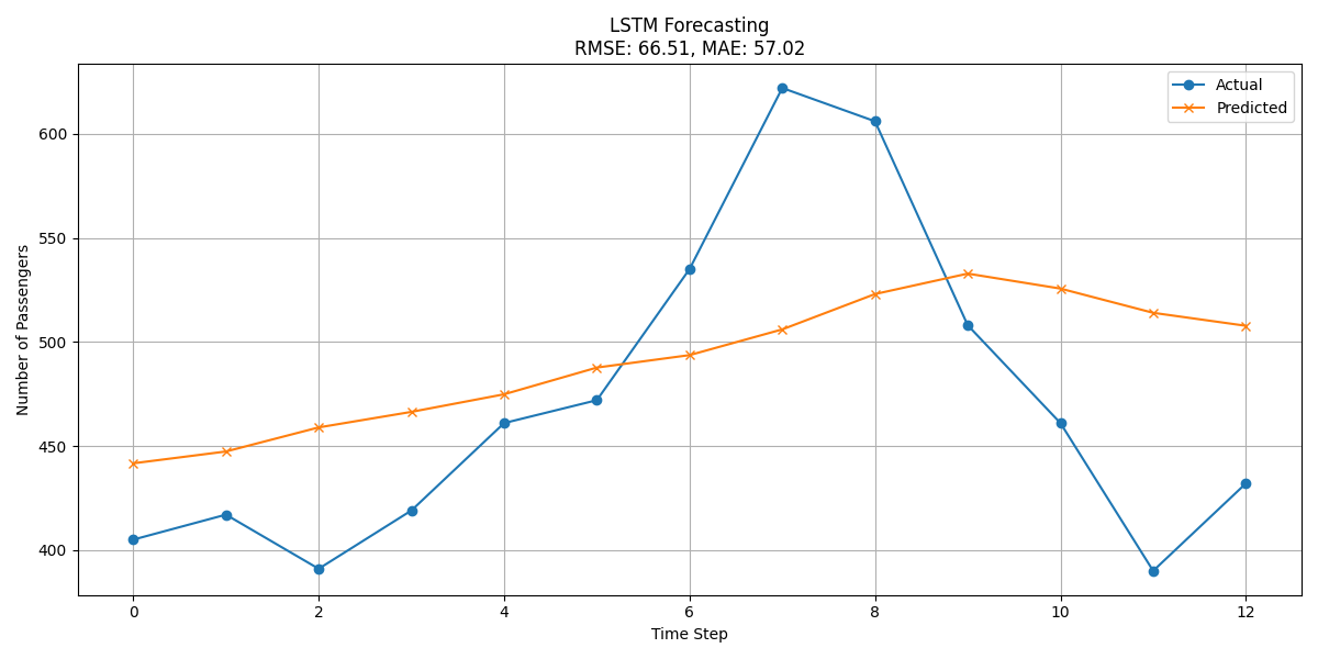
plt.figure(figsize=(12, 6))
plt.plot(y_test_inv, label='Actual', marker='o')
plt.plot(y_pred_inv, label='Predicted', marker='x')
plt.title(f'LSTM Forecasting\nRMSE: {rmse:.2f}, MAE: {mae:.2f}')
plt.xlabel('Time Step')
plt.ylabel('Number of Passengers')
plt.legend()
plt.grid(True)
plt.tight_layout()
plt.savefig('LSTM_forecasting.png')
plt.show()